STOP TAKING DIFFERENTIAL EQUATIONS

Just read this article instead

Posted Nov 8, 2026

By Samuel Lowe 45 min read

At Northeastern University, students pursuing a math minor were required to take two out of these three courses:

Multivariable and Vector Calculus, starting with partial derivatives and ending with the three-dimensional statement of Stokes’ theorem,
Linear Algebra, introducing vector spaces and reduced row-echelon form and ending with singular value decomposition and other applications, and
Linear Algebra and Ordinary Differential Equations, introducing linear ordinary differential equations (ODEs) and matrix math and ending with the Laplace transform and the eigenvalue method for systems of linear ordinary differential equations.

These are more or less standard classes for American undergrads: they’re geared towards engineers and don’t present any proofs.

After taking all three, I (and most other math majors) made a point to always recommend the first two courses and actively dissuade anyone from taking the third. Linear Algebra and Ordinary Differential Equations sounds promising, seemingly covering two courses’ worth of material for the price of one; but anyone who took a standard linear algebra course could self-teach the entire course in an afternoon, provided they had a good resource.

This article is that resource. It won’t teach the entire syllabus, but that’s because most of it is obsolete by the end of the course. We’ll learn the stuff that isn’t obsolete by the end, point out which topics we’re omitting (all of which are methods), and supplement the material with some additional details that hopefully make our theory of ordinary differential equations a bit clearer and deeper.

Accessibility

This article expects a solid understanding of linear algebra (up to eigenvectors and eigenvalues) and familiarity with calculus, preferably up to integration by parts. Knowledge of Jordan canonical form will be useful to see a method in more generality, but is entirely optional.

What’s a Differential Equation?

A differential equation is an equation that defines an unknown function in terms of its derivatives. We call a differential equation ordinary (an “ODE”) when the function we’re working with takes only a single input variable $x$ (some authors prefer $t$). We typically denote this unknown function $y$ (the authors who use $t$ for the independent variable might use $x$ to refer to the function).

We say the order $n$ of the differential equation is the highest order derivative $y^{(n)}$ that appears in the equation. A solution to an ordinary differential equation $E$ is an $n$-times continuously differentiable function $y : I \to \F$ satisfying $E$ on the interval $I$, where $\F$ is either $\R$ or $\C$.

Example

The most famous ordinary differential equation is probably

\[y^\prime = y \tag{$E$}\]

The order of this equation $E$ is $n = 1$ because the highest derivative is $y^\prime = y^{(1)}$. Its solutions take the form $y(x) = Ce^x$ for any constant $C \in \C$.

Example

You can also consider the equation

\[y^\prime = y - x \tag{$E$}\]

This is again a first-order equation; the $x$ doesn’t affect the order. The solutions of this equation take the form $y(x) = Ce^x + x + 1$ for any constant $C \in \C$.

We often specify additional requirements, known as initial conditions, on $y$. For example, if we specify $y(0) = 1$ in the first example, $y^\prime=y$, then we no longer have a free coefficient $C$: the initial condition forces $C = 1$ and our solution to be $y(x) = e^x$.

Example

Consider the second-order equation

\[y^{\prime\prime} = -y\]

We say second-order because the highest derivative is $y^{\prime\prime} = y^{(2)}$ (hence the order $n = 2$). Its solutions take the form $y(x) = C_1\sin(x) + C_2\cos(x)$ for constants $C_i \in \C$.

If we specify initial conditions $y(0)=1$ and $y^\prime(0)=2$, then $C_2=1$ and $C_1=2$, so the solution becomes $y(x)=2\sin(x)+\cos(x)$.

Example

Consider

\[y^{\prime\prime} = y - x^2\]

The order of this equation is $n = 2$ because the highest derivative is $y^{\prime\prime} = y^{(2)}$. Its solutions take the form $y(x) = C_1e^x + C_2e^{-x} + x^2 + 2$ for constants $C_i \in \C$. Fitting this solution to the initial conditions $y(0) = 1$ and $y^{\prime}(0) = 1 + i$ gives $C_1+C_2=-1$ and $C_1-C_2=1+i$, so $C_1 = i/2$ and $C_2 = -1-i/2$, and the solution becomes

\[y(x) = \frac{i}{2}e^x - \left(1+\frac{i}{2}\right)e^{-x} + x^2 + 2\]

However, if we had been given $y(0) = 2$ and $y^{\prime}(0) = 0$, then we would get

\[y(x) = x^2 + 2\]

since $C_1 = C_2 = 0$.

For now, you don’t need to know how to actually obtain these solutions, but you should be able to verify the solutions I’ve provided by differentiating and plugging in. We’ll discuss how we can find these solutions shortly.

The general form of a linear $n$-th order ordinary differential equation is the linear combination

\[c_n(x)y^{(n)} + \cdots + c_1(x)y^\prime + c_0(x)y = f(x)\]

with $c_n(x)\neq 0$ throughout the interval on which we work. That function $f(x)$ is called the forcing term; a linear ODE whose forcing term is not identically zero is called inhomogeneous, and a linear ODE whose forcing term is identically zero is called homogeneous.

Here, linear means that $y$ and its derivatives appear only in a linear combination: there are no squares like $y^2$ or products like $yy^\prime$. The coefficients may depend on $x$, but not on $y$ or its derivatives. For example, $y^\prime=y-x$ is linear, while $y^\prime=y^2$ is nonlinear.

In this article, we’re going to be focusing only on linear ODEs with constant coefficients, so each $c_i$ is a constant:

\[c_ny^{(n)} + \cdots + c_1y^\prime + c_0y = f(x)\]

Why only constant coefficients?

Almost all of the solution-set theorems we state will also work for linear ODEs with non-constant coefficients, provided each $c_i(x)$ and the forcing term are continuous functions and $c_n(x) \neq 0$ throughout the interval. The problem is that the two solution methods we develop below don’t generally work in the same way when we allow non-constant coefficients, so for consistency we’re going to restrict the stated theorems to constant coefficients as well. We’ll cover the more general theorems and the issues they cause in the solution methods in an aside towards the end of the article.

Existence and Uniqueness of Solutions

Before we start hunting around for solutions to these equations, we should verify that they actually exist in the first place! Rest assured, solutions to well-behaved ODEs always exist, at least locally, thanks to a theorem known as Picard–Lindelöf. Here’s a special case for linear ordinary differential equations with constant coefficients:

Theorem (Existence and Uniqueness of Solutions to Ordinary Differential Equations)

Let $I \subseteq \R$ be an open interval, let $f : I \to \C$ be continuous, and let $c_0,\ldots,c_n \in \C$ be constants with $n \ge 1$ and $c_n \neq 0$. For any initial point $x_0 \in I$ and initial values $b_0,\ldots,b_{n-1} \in \C$, the equation

\[c_ny^{(n)}+\cdots+c_1y^\prime+c_0y=f(x)\]

has exactly one $n$-times continuously differentiable solution $y : I \to \C$ satisfying the initial conditions

\[y^{(k)}(x_0)=b_k, \qquad 0 \le k<n\]

Proof

We could prove the result by induction, but we opt for a slightly longer route (that is the same in spirit) to present an explicit algorithm that constructs the unique solution.

$(n = 1)$ Consider the first-order equation
\[u^\prime-ru=g(x), \qquad u(x_0)=a,\]
with constant $r \in \C$ and continuous forcing $g$. Multiplying by the integrating factor $e^{-rx}$ turns the left side into the derivative of $e^{-rx}u(x)$. Integrating and rearranging gives
\[u(x)=e^{r(x-x_0)}a+\int_{x_0}^x e^{r(x-t)}g(t)\,dt.\]
The fundamental theorem of calculus uniquely determines a function on an interval from its derivative and its value at one point, so every solution must have the above form. Differentiating verifies that this is a valid solution. Thus this first-order problem has exactly one solution on all of $I$.
$(n > 1)$ Here, some algebraic trickery (that we must regrettably wait until later to properly motivate) provides an algorithm to construct a solution, and we then justify that the algorithm must produce the unique solution.
For the $n$-th order equation
\[c_ny^{(n)}+\cdots+c_1y^\prime+c_0y=f(x) \tag{$E$}\]
we consider the characteristic polynomial $p(s)$ of $E$, where a derivative $c_ky^{(k)}$ of order $k$ corresponds to a polynomial term $c_ks^k$ in the variable $s$.
\[p(s) := c_ns^n+\cdots+c_1s+c_0\]
(We’ll justify that this correspondence actually encodes meaningful information in the section below on the Laplace transform; for now, it should suffice to see that it’s a well-defined bijection between the linear combinations of all derivatives in an equation and polynomials of degree $n$.) Factoring over $\C$,
\[p(s) = c_n(s-r_1)\cdots(s-r_n)\]
(where roots are listed with multiplicity), we can recursively define the auxiliary functions:
\[z_0=y, \qquad z_j=z_{j-1}^\prime-r_jz_{j-1}, \qquad 1\le j\le n\]
Expanding these expressions reproduces the coefficients of the factored polynomial $p(s)$, so the original equation is equivalent to $z_n=f/c_n$. For example, the first two steps give
\[z_1=y^\prime-r_1y, \qquad z_2=y^{\prime\prime}-(r_1+r_2)y^\prime+r_1r_2y.\]
In general, $z_j$ is $y^{(j)}$ plus a fixed linear combination of lower derivatives. The prescribed values $b_0,\ldots,b_{n-1}$ therefore determine initial values $a_j=z_j(x_0)$ for $0\le j<n$. Conversely, each $a_j$ determines the original initial derivatives.
Starting with the known function $z_n=f/c_n$, back-solving the first-order problems
\[z_{j-1}^\prime-r_jz_{j-1}=z_j, \qquad z_{j-1}(x_0)=a_{j-1}, \qquad j=n,n-1,\ldots,1\]
gives exactly one function on $I$. Each step also adds one continuous derivative: $z_n$ is continuous, so $z_{n-1}$ is continuously differentiable, and eventually $z_0=y$ is $n$-times continuously differentiable. By construction, it satisfies the original equation and all the prescribed initial conditions. This proves existence.
Uniqueness is simple: any other solution would produce the same auxiliary initial values and have to solve the same sequence of first-order problems, and from our $n = 1$ case we know that those must be solvable uniquely. Any other solution therefore gives the same $y$, so we conclude that it’s unique.

The above algorithm given in the general case produces a solution and guarantees uniqueness by construction. Unfortunately, this method is quite tedious: it demands that we factor an $n$-th degree polynomial, then complete a sequence of $n$ integrating factor integrals. We’ll introduce more convenient methods shortly.

We conclude with a remark about the existence of real solutions. If the coefficients, forcing, and initial values are all real, complex conjugation gives another solution with the same initial values. Uniqueness therefore forces $y=\overline y$, so the solution is real-valued; we’ll leverage this to produce real solutions from complex ones in a later section.

A neat corollary of this is Euler's identity. Consider the differential equation

\[y^\prime = iy, \quad y(0) = 1\]

You can verify that $y(x) = e^{ix}$ is a solution of this equation with the prescribed initial value. However, $\cos(x) + i\sin(x)$ is also a solution with that initial value. If these functions were different, then we would contradict the uniqueness of solutions to ordinary differential equations, so these functions must be the same. This equality is known as Euler's formula:

\[e^{ix} = \cos(x) + i\sin(x)\]

and the above argument constitutes a valid (if informal) proof. Plugging in $x = \pi$ and adding $1$ to both sides, we obtain Euler’s identity:

\[e^{i\pi} + 1 = 0\]

Solving Equations

Now that we know solutions exist, we should discuss how to find them.

Courses teach a variety of methods:

Separation of variables, which is useful for nonlinear ODEs like $y^\prime = y^2$, but nonlinear ODEs were rarely discussed in my course.
Guess-and-check, where we simply make a guess, like
\[y \relatedby{?}{=} C_1\sin(\lambda_1x) + C_2\cos(\lambda_2x) + C_3e^{\lambda_3x}\]
or something similarly tedious, then differentiate as many times as required, plug our guesses for $y$ into the original equation $E$, then solve the resulting equations for the values of $C_i$ and $\lambda_i$.
Power series, where we assume that $y$ is analytic near the initial point (say $x=0$), and has a power series
\[y = \sum_{m=0}^\infty a_mx^m\]
We plug this in and solve recursively for the coefficients $a_m$, then hope to recognize the solution. For a linear ODE, analytic coefficients and forcing near the initial point, with a nonzero leading coefficient there, guarantee this local analyticity; continuity alone doesn’t. This also works for linear ODEs with non-constant coefficients, though the series may only converge locally, and gets messy fast for nonlinear equations with products of derivatives of $y$.

But again, my undergraduate course restricted most of its attention to linear equations with constant coefficients. For those examples, much of the above became busywork once we had simpler and more systematic methods like the two we discuss below. The other methods still have uses outside that setting.

In a general linear ordinary differential equation $E$, the forcing term is probably nonzero:

\[c_ny^{(n)}+\cdots+c_1y^\prime+c_0y=f(x). \tag{$E$}\]

If it’s true that $f(x)$ isn’t identically zero, then a solution to $E$ is called a particular solution $y_p$. There is a similar homogeneous equation called the associated homogeneous differential equation $E_h$

\[c_ny^{(n)}+\cdots+c_1y^\prime+c_0y=0 \tag{$E_h$}\]

obtained by setting $f(x) = 0$; solutions to $E_h$ are called homogeneous solutions (or modes in some settings).

By substitution, adding $y_p$ to any homogeneous solution $y_h$ of $E_h$ gives a solution of $E$, and subtracting $y_p$ from any solution of $E$ gives a solution of $E_h$. Thus every solution has the form

\[y=y_h+y_p\]

and a formula covering every solution is called a general solution. We’ll explain the structure of these solutions after we see how to obtain them in the first place.

The Laplace Transform

As tedious as that power series method is, it’s well-suited to solving a large class of ODEs. It would be nice if we had a method that was just as powerful, but less obnoxious to compute.

It turns out we can derive one by making the power series idea continuous. A power series takes a sequence of numbers $a(0),a(1),a(2),\ldots$ and packages it into a single function of a new variable $t$:

\[\sum_{m=0}^\infty a(m)\,t^m=A(t).\]

Here $a$ is a function of a discrete variable $m=0,1,2,\ldots$. Suppose we instead have a function $f(x)$ of a continuous variable $x\ge0$. The continuous analog of a sum is an integral, so the analogous construction is

\[\int_0^\infty f(x)\,t^x\,dx.\]

For this integral to have any hope of converging, $t^x$ should decay as $x\to\infty$, so we want $0<t<1$. Powers of an arbitrary base are awkward to integrate and differentiate, so we rewrite $t$ in base $e$ as $t=e^{-s}$, where $0<t<1$ corresponds to $s>0$. Then $t^x=e^{-sx}$, and we arrive at

\[\int_0^\infty f(x)e^{-sx}\,dx.\]

This is the Laplace transform: a continuous power series, with $f(x)$ playing the role of the coefficients.

Definition (Laplace Transform)

The Laplace transform of a piecewise continuous function $f$ on $[0,\infty)$ is

\[\Laplace{f}(s) := \int_0^\infty e^{-sx}f(x)\,dx,\]

for those $s\in\C$ where the integral converges.

Conventionally, we write $Y(s)=\Laplace{y}(s)$ and $F(s)=\Laplace{f}(s)$ and call the original domain (in $x$) the time domain and the transformed domain (in $s$) the frequency domain, even when $x$ represents something other than time.

Is this related to the Fourier transform?

Well, everything is related to the Fourier transform if you look hard enough, but in this case the Laplace transform actually is the Fourier transform, just with a handful of changes so more functions converge.

More precisely, the Laplace transform is the Fourier transform of $f$ after cutting it off to $x \geq 0$ and damping it by $e^{-\sigma x}$:

\[\Laplace{f}(\sigma + 2\pi i \xi) = \int_0^\infty f(x)e^{-\sigma x}e^{-2\pi i \xi x}\,dx = \hat g_\sigma(\xi), \qquad g_\sigma(x) = f(x)e^{-\sigma x}\mathbf{1}_{[0,\infty)}(x)\]

Applying Fourier inversion to $g_\sigma$ and multiplying back by $e^{\sigma x}$ gives the integral in the Laplace inversion theorem, called the Bromwich inversion integral, which gives us $f(x)$ from $F(s)$ for $x > 0$.

Alternatively, you can consider the Fourier transform as the two-sided Laplace transform restricted to the imaginary axis: $\hat f(\xi) = \mathcal{B}f(2\pi i \xi)$, where $\mathcal{B}f(s) = \int_{-\infty}^\infty f(x)e^{-sx}\thinspace dx$.

We can also see that the Laplace transform captures frequency data by splitting $s=\sigma+i\omega$, which decomposes $e^{-sx}$ into the exponential damping at rate $\sigma$ times an oscillation with angular frequency $\omega$:

\[e^{-sx}=e^{-\sigma x}e^{-i\omega x}\]

One more connection to the Fourier transform becomes obvious when solving partial differential equations, where we typically want to solve for a function that has multiple independent input variables rather than just one. A common setup is to solve for a function $u(\mathbf{x}, t)$, where $\mathbf{x} = (x, y, z)$ represents a position in space and $t$ represents a position in time. Ordinary differential equations, on the other hand, typically represent some kind of system as it evolves over time. (That’s why the independent variable is often written $t$ instead of $x$ as in this article.)

If such a PDE is linear with constant coefficients, it has the form

\[P\left(\frac{\partial}{\partial t}, \frac{\partial}{\partial x}, \frac{\partial}{\partial y}, \frac{\partial}{\partial z}\right) u = f(\mathbf{x}, t)\]

where $P$ is a polynomial in those four variables with constant coefficients: “multiplying” these variables is composing their partial derivative operations, so “squaring” the variable $\partial/\partial x$ gives us the second partial derivative $\partial^2/\partial x^2$ in $x$, cubing gives us $\partial^3/\partial x^3$, and so on. “Multiplication” between different variables is commutative by Clairaut’s theorem.

Examples abound:

The heat equation $\frac{\partial u}{\partial t} = k \nabla^2 u$, which models how temperature spreads through a uniform material
The wave equation $\frac{\partial^2 u}{\partial t^2} = c^2 \nabla^2 u$, which models waves like sound traveling at speed $c$
The Laplace equation $\nabla^2 u = 0$, which models steady states, like the temperature in a material after it has stopped changing
The Poisson equation $\nabla^2 u = f(\mathbf{x})$, which models the gravitational or electric potential $u$ produced by a density $f$ of mass or charge
The advection equation $\frac{\partial u}{\partial t} + \mathbf{v} \cdot \nabla u = 0$, which models a substance with concentration $u$ being carried along by a current with constant velocity $\mathbf{v}$

These equations can be solved by taking successive Fourier transforms for each spatial variable, and a Laplace transform if there’s a temporal variable $t$, solving the resulting algebra problem, then transforming back to obtain our solution $u$. The Fourier transform in $x$ turns $\frac{\partial}{\partial x}$ into multiplication by $2\pi i \xi_1$ (and likewise for $y$ and $z$ with $\xi_2$ and $\xi_3$), and the Laplace transform turns $\frac{\partial}{\partial t}$ into multiplication by $s$ plus initial-value terms, just as it did for ODEs. Writing $U(\boldsymbol{\xi}, s)$ and $F(\boldsymbol{\xi}, s)$ for the transformed $u$ and $f$, the PDE becomes

\[P(s, 2\pi i \xi_1, 2\pi i \xi_2, 2\pi i \xi_3)\, U(\boldsymbol{\xi}, s) = F(\boldsymbol{\xi}, s) + (\text{initial-value terms})\]

so solving for $U$ just means dividing by a polynomial.

This works as long as the problem is posed on all of $\R^3 \times [0, \infty)$, since the Fourier transform integrates over all of $\R^3$. On a bounded region like a box, we use Fourier series instead.

There’s one catch. A power series only converges if its coefficients don’t grow too quickly: if there exist $M, \rho > 0$ such that $\lvert a(m)\rvert\le M\rho^m$, then the comparison test tells us the series converges for $\lvert t\rvert<1/\rho$.

The continuous analog for our integral is needing $e^{-sx}$ to decay faster than $f$ grows. One simple and quite permissive condition is that $f$ be of exponential order:

Definition (Exponential Order)

We say a function $f: [0, \infty) \to \C$ is of exponential order if there exist real numbers $M > 0$ and $a$ such that

\[\lvert f(x)\rvert\le Me^{ax}\]

for all $x \geq 0$.

Exponential Order and Big O Notation

For piecewise continuous $f$, we can express exponential order in big O notation (explicitly stating the requirement that this holds as $x \to \infty$, which is left implicit in fields like computer science):

\[\lvert f(x) \rvert \leq e^{\mathcal{O}(x)} \quad \text{as } x \to \infty\]

If we prefer to make the existence of some real $a$ explicit, we can express the statement in both big O notation and little o notation as:

\[f(x) = \mathcal{O}(e^{ax}) \quad \text{as } x \to \infty\] \[f(x) = o(e^{ax}) \quad \text{as } x \to \infty\]

(although the $a$ in each statement may differ).

When $f$ is of exponential order,

\[\lvert f(x)e^{-sx}\rvert\le Me^{-(\Re(s)-a)x}\]

so the integral converges absolutely whenever $\Re(s)>a$, or equivalently $0< \lvert t \rvert < e^{-a}$. This is analogous to a radius of convergence.

Which functions have a Laplace transform?

As hinted at previously, the requirement that $f(x)$ be of exponential order is slightly stronger than is necessary for a Laplace transform to exist. We can lay out more general criteria for a function $f$ to be Laplace transformable in the language of functional analysis:

Definition ($L^1(\Omega)$)

Let $\Omega$ be a real interval. The set of all absolutely integrable functions on $\Omega$ is

\[L^1(\Omega) := \setbuild{f(x)}{\int_\Omega |f(x)| \, dx < \infty}\]

$L^1$ is pronounced “ell one”.

(This set is actually just one example of an $L^p$ space. For $1 \leq p \leq \infty$, $L^p$ is an infinite-dimensional vector space, a metric space, and — if we’re taking integrals using the Lebesgue integral — is also complete in the same way that the real numbers are: Cauchy sequences of functions in $L^p$ converge very nicely just like Cauchy sequences of real numbers do. In the more abstract field of measure theory, $\Omega$ just has to be a measurable set.)

We can now describe Laplace transformability much more broadly:

Theorem (Laplace Transformability)

A function $f: [0, \infty) \to \C$ is Laplace transformable if there exists some real $\sigma$ such that

\[f(x)e^{-\sigma x} \in L^1[0, \infty)\]

If even one $\sigma$ exists, then there are infinitely many, and they form an interval

\[(\sigma_{\mathrm{inf}}, \infty) \text{ or possibly } [\sigma_{\mathrm{inf}}, \infty)\]

where $\sigma_{\mathrm{inf}}$ may be $-\infty$ (in which case every real $\sigma$ works). The Laplace integral defining $F(s)$ converges absolutely on the half-plane $\Re s > \sigma_{\mathrm{inf}}$ (and possibly on its entire boundary line $\Re s = \sigma_{\mathrm{inf}}$), and $F$ is holomorphic (complex-differentiable) on that open half-plane.

This slightly relaxes our previous exponential order requirement to allow more functions, like $f(x)=1/\sqrt{x}$. This function blows up at $x=0$, so no bound $Me^{ax}$ holds near $0$, but it’s still integrable there, and $\Laplace{x^{-1/2}}(s)=\sqrt{\pi/s}$.

So this simultaneously includes integrable singularities like $1/\sqrt{x}$ at $x = 0$ and correctly excludes non-integrable singularities like $1/x$ at $x=0$ and other bad behavior that would cause $F(s)$ to misbehave.

Just as $A(t)$ encodes the entire sequence $a(m)$ in one function, the Laplace integral encodes all of $f$ in one function $F(s)$, so we can recover $f$ from it via the Laplace inversion theorem:

Theorem (Laplace Inversion)

Suppose $f$ is continuous on $[0,\infty)$, continuously differentiable on $(0,\infty)$, and of exponential order with $\lvert f(x)\rvert\le Me^{ax}$, and let $F=\Laplace{f}$. Then for every real $\gamma>a$ and every $x>0$,

\[f(x)=\frac{1}{2\pi i}\lim_{T\to\infty}\int_{\gamma-iT}^{\gamma+iT}F(s)e^{sx}\,ds,\]

where the integral runs up the vertical line $\Re(s)=\gamma$. A related result, Lerch's theorem, says that two continuous functions of exponential order with the same Laplace transform are equal, even without the differentiability assumption.

For this method, we’ll work forwards from the initial point on a half-line, so shift the independent variable to put the initial point at $x=0$. We only require that the forcing be continuous on $[0,\infty)$ and of exponential order. For constant-coefficient equations, the solution and its derivatives through order $n$ are then of exponential order too, possibly with a larger $a$.

The transform is linear because integration is linear. Here is the correspondence that makes it useful:

Theorem (Constant-Coefficient ODEs under the Laplace Transform)

Let $y$ be an $n$-times continuously differentiable function on $[0,\infty)$ such that $y$ and its first $n$ derivatives $y^\prime, \ldots, y^{(n)}$ are of exponential order, and let $b_j=y^{(j)}(0)$ denote the initial values. For $1\le k\le n$, the Laplace transform of $y^{(k)}$ is

\[\Laplace{y^{(k)}}(s)=s^kY(s)-\sum_{j=0}^{k-1}s^{k-1-j}b_j.\]

Summing these transforms from $0$ to $n$, we see that, for continuous forcing $f$ of exponential order, the constant-coefficient equation

\[\sum_{k=0}^n c_ky^{(k)}=f(x), \qquad c_n\neq 0,\]

corresponds to the algebraic equation

\[p(s)Y(s)=F(s)+Q(s),\]

where

\[p(s)=\sum_{k=0}^n c_ks^k, \quad Q(s)=\sum_{k=1}^n c_k\sum_{j=0}^{k-1}s^{k-1-j}b_j, \quad F(s) = \Laplace{f}(s)\]

These identities hold for sufficiently large $\Re(s)$. In particular, when all the initial values are zero, the correspondence is simply $p(s)Y(s)=F(s)$.

This theorem might seem quite complicated, but if you work through even one or two examples it becomes screamingly obvious — so obvious in fact that it became the first theorem I ever wanted to prove on my own!

Proof

We proceed by induction on the order $k$ of the derivative term $y^{(k)}$.

$(k = 1)$ Integrating $\Laplace{y^\prime}$ by parts gives
\[\begin{aligned} \Laplace{y^\prime}(s) &=\lim_{R\to\infty}\int_0^R e^{-sx}y^\prime(x)\,dx\\ &=\lim_{R\to\infty}\left(e^{-sR}y(R)-y(0) +s\int_0^R e^{-sx}y(x)\,dx\right)\\ &=\lim_{R\to\infty}\left(e^{-sR}y(R)\right) + s\lim_{R\to\infty}\left(\int_0^R e^{-sx}y(x)\,dx \right) - y(0)\\ &=\lim_{R\to\infty}\left(e^{-sR}y(R)\right) + sY(s) - y(0) \end{aligned}\]
Because $y$ is of exponential order and $\Re(s)$ is larger than the $a$ in its bound, the boundary term at infinity vanishes, and we obtain
\[\begin{aligned} \Laplace{y^\prime}(s) &=\underbrace{\lim_{R\to\infty}\left(e^{-sR}y(R)\right)}_{\to 0} + sY(s) - y(0)\\ &=sY(s)-y(0) \end{aligned}\]
as desired.
$(k - 1 \implies k)$ Applying the same calculation to each successive derivative gives the recurrence
\[\Laplace{y^{(k)}}(s) = s\Laplace{y^{(k-1)}}(s)-b_{k-1}\]
The inductive hypothesis gives the stated derivative formula. By linearity, transforming the full equation therefore gives
\[\begin{aligned} F(s) &=c_0Y(s)+\sum_{k=1}^n c_k\left(s^kY(s)-\sum_{j=0}^{k-1}s^{k-1-j}b_j\right)\\ &=p(s)Y(s)-Q(s) \end{aligned}\]
Rearranging yields the desired formula.

This correspondence also works in reverse: if $y$ and its derivatives satisfy the exponential order requirement, $y$ has the prescribed initial values, and its transform satisfies this algebraic equation, then the transform of the residual

\[\sum c_ky^{(k)}-f\]

is zero. By Lerch’s theorem (which we use here without proof), that residual is identically zero.

Notice that the coefficients of the derivatives become the coefficients of the characteristic polynomial $p(s)$ from the existence proof. The transformed solution $Y$ and forcing $F$ need not be polynomials.

Okay, so what’s the big picture here? The idea is that solving a differential equation directly is usually quite complicated, but the Laplace transform reduces it down to an associated algebra problem:

Rearranging the formula in the theorem above, the solution to the algebraic equation is

\[Y(s)=\frac{F(s)+Q(s)}{p(s)}.\]

The only complicated part is factoring the characteristic polynomial $p(s)$, then doing the inverse Laplace transform to recover $y$. For rational expressions (that is, when $F$ is rational), this just turns into a partial fractions problem, whose terms have well-known inverse transforms that we can just look up in a table.

For example, direct integration gives

\[\Laplace{e^{rx}}(s)=\frac{1}{s-r},\]

and repeated integration by parts gives the more general pair

\[\Laplace{x^m e^{rx}}(s)=\frac{m!}{(s-r)^{m+1}}, \qquad m=0,1,2,\ldots.\]

Both formulas hold for $\Re(s)>\Re(r)$. Other common pairs are collected in transform tables; inversion doesn’t always reduce to elementary functions.

Perhaps some examples will make this concrete:

Example

Consider

\[y^{\prime\prime}-3y^\prime+2y=e^{3x}, \qquad y(0)=y^\prime(0)=0\]

The initial-value terms are zero, so transforming gives

\[(s^2-3s+2)Y(s)=\frac{1}{s-3}\]

Factoring and using partial fractions:

\[\begin{aligned} Y(s)&=\frac{1}{(s-1)(s-2)(s-3)}\\ &=\frac{1}{2(s-1)}-\frac{1}{s-2}+\frac{1}{2(s-3)} \end{aligned}\]

Taking the inverse transform term by term gives

\[y(x)=\frac12e^x-e^{2x}+\frac12e^{3x}.\]

Example

For the same equation with nonzero initial values $y(0)=1$ and $y^\prime(0)=1$, the derivative formulas give

\[\begin{aligned} (s^2Y-s-1)-3(sY-1)+2Y&=\frac{1}{s-3},\\ (s^2-3s+2)Y&=\frac{1}{s-3}+s-2 \end{aligned}\]

Here $Q(s)=s-2$. Dividing gives

\[Y(s)=\frac{1}{(s-1)(s-2)(s-3)}+\frac{1}{s-1}\]

That nonzero $Q(s)/p(s)$ term means that when we run everything through the inverse Laplace transform, we get an extra $e^x$ compared to the above example:

\[y(x)=\frac32e^x-e^{2x}+\frac12e^{3x}\]

To find a general solution instead, leave the initial values $b_j$ as free parameters. Alternatively, set them all to zero to obtain one particular solution, then add the general homogeneous solution as before.

Real Solutions from Complex Solutions

When the coefficients, forcing term, and initial values are all real, we can obtain a real-valued solution (as the end of the existence proof shows), which is frequently what we want to do in real-world applications; otherwise, we may need complex-valued solution functions $I \to \C$. Even in the real case, we may have to detour through $\C$, but we just have to know how to find our way out.

(The theory also has a complex-analytic version, with a complex independent variable on a fixed open disk $B \subseteq \C$, provided the forcing term is complex analytic. For real-life applications (which undergrad diffeq classes prioritize), we typically use a real independent variable $x$, so we work on a fixed open interval $I \subseteq \R$.)

Consider

\[y^{\prime\prime}+y=0\]

which has characteristic roots $i$ and $-i$. The general complex solution is $C_1e^{ix}+C_2e^{-ix}$.

If these solutions don’t look real to you, recall Euler’s formula

\[e^{(a+bi)x}=e^{ax}\cos(bx)+i e^{ax}\sin(bx)\]

and the theorem that the non-real roots of real polynomials come in conjugate pairs $a \pm bi$. Putting this together, we see

\[\begin{aligned} e^{ix}&=\cos(x)+i \sin(x)\\ e^{-ix}&=\cos(-x)+i \sin(-x)\\ &=\cos(x)-i \sin(x) \end{aligned}\]

where $\sin$ being odd and $\cos$ being even allow the second equality. Adding and subtracting these solutions gives

\[\begin{aligned} e^{ix}+e^{-ix}&=2\cos(x)\\ e^{ix}-e^{-ix}&=2i\sin(x) \end{aligned}\]

Because sums and multiples of homogeneous solutions are still solutions, if we were forced to keep the $2$ and $2i$ leading coefficients (we’re not, and you’ll see why), we could always choose a coefficient for $2i\sin(x)$ that causes the $i$ to cancel. In terms of our general solution, $C_1e^{ix}+C_2e^{-ix}=D_1^\ast\,2\cos(x)+D_2^\ast\,2i\sin(x)$, where $D_1^\ast=(C_1+C_2)/2$ and $D_2^\ast=(C_1-C_2)/2$, so we can absorb the $2$ and $2i$ into new coefficients:

This is why we’re not forced to keep the $2$ and $2i$ in front; these coefficients are completely interchangeable. The thing that matters is preserving the relationship between all $x$ terms within $\sin(x)$ and $\cos(x)$’s Taylor series; any linear combination of $\sin(x)$ and $\cos(x)$ (even with one or both coefficients $0$) is a valid solution. In particular, dropping the $2$ and $2i$ still preserves that relationship, so we’re in good shape to choose real $D_1$ and $D_2$.

This example contains the general method:

Identify the complex conjugate pairs.
For each conjugate pair $a \pm bi$ with multiplicity $m \geq 1$, make the substitutions via Euler:
\[x^ke^{(a\pm bi)x} \mapsto x^ke^{ax}\cos(bx), x^ke^{ax}\sin(bx)\]
for $0\le k<m$. The $x^k$ terms correct for multiplicity.
Absorb the constant factors (like the $2$ and $2i$ above) into new free coefficients, which we can restrict to $\R$ if we’d like.

Isn’t that neat?

Resonance

Solution methods may encounter difficulties if the forcing term contains an exponential $e^{rx}$ that also shows up as a solution to the homogeneous equation. For example,

\[y^{\prime\prime}-3y^\prime+2y=e^x\]

has characteristic roots $1$ and $2$, so $e^x$ is a homogeneous solution. The forcing is $e^x$, so we’d naturally guess a particular solution $y=Ae^x$. Plugging it in gives

\[Ae^x-3Ae^x+2Ae^x=0\]

no matter what $A$ is, so no multiple of $e^x$ can be a particular solution! What’s going on here?

This phenomenon is called resonance. The fix is simple: multiply the guess by $x$. Trying $y=Axe^x$ gives $y^\prime=A(x+1)e^x$ and $y^{\prime\prime}=A(x+2)e^x$, so

\[A(x+2)e^x-3A(x+1)e^x+2Axe^x=-Ae^x\]

The $x$ terms cancel, so $A=-1$ and the general solution is $y=C_1e^x+C_2e^{2x}-xe^x$. If $r$ is a repeated root of multiplicity $k$, so that $e^{rx},xe^{rx},\ldots,x^{k-1}e^{rx}$ are all homogeneous solutions, multiply by $x^k$ instead. For example, $y^{\prime\prime}-2y^\prime+y=e^x$ has the double root $1$ and the particular solution $\frac12x^2e^x$.

What’s actually going on here?

When our forcing contains an exponential $e^{rx}$ that is already a homogeneous solution, $r$ is a root of the characteristic polynomial, so $p(r)=0$. Dividing $F(s)$ by $p(s)$ then creates a higher-order version of a type of asymptote called a pole at $s=r$ in our solution’s Laplace transform $Y(s)$:

Definition (Pole)

Let $F$ be holomorphic (that is, complex-differentiable) on a punctured disk $0<\lvert s-r\rvert<\varepsilon$ around a point $r\in\C$. Then $F$ has a pole at $r$ if $\lvert F(s)\rvert\to\infty$ as $s\to r$.

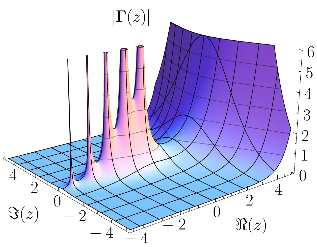A visualization of the absolute value of the gamma function, which has several poles sticking up along the non-positive integers. Geek3, CC BY-SA 3.0 https://creativecommons.org/licenses/by-sa/3.0, via Wikimedia Commons

In that case, there is a unique positive integer $k$, called the order of the pole, such that

\[F(s)=\frac{g(s)}{(s-r)^k}\]

for some function $g$ that is holomorphic on the whole disk $\lvert s-r\rvert<\varepsilon$ with $g(r)\neq0$.

For example, $1/(s-r)$ has a pole of order one, while $1/(s-r)^2$ has a pole of order two. The inverse Laplace transform sends these functions to $e^{rx}$ and $xe^{rx}$, respectively. In general, the inverse Laplace transform takes a pole of order $j$ at $s=r$ to $x^{j-1}e^{rx}$, up to a constant factor. Accordingly, we have to multiply our guess by $x$.

Repeated roots work the same way. If $r$ is a root of $p$ with multiplicity $k$, then $p(s)$ contributes a factor of $(s-r)^k$ to the denominator of $Y(s)$, and forcing by $e^{rx}$ contributes one more. The resulting pole of order $k+1$ inverts to a multiple of $x^ke^{rx}$, plus lower powers of $x$ times $e^{rx}$ that are already homogeneous solutions.

Example (Resonance in Saturn’s Rings)

Saturn eclipsing the Sun, seen from behind by the Cassini orbiter in 2006. NASA/JPL/Space Science Institute, public domain, via Wikimedia Commons

The speed at which particles in Saturn’s rings orbit is determined by their distance from Saturn. Kepler’s third law tells us that closer particles orbit faster, and farther particles orbit slower.

Saturn’s B ring stops abruptly around 117,500 kilometers from Saturn’s center. As it turns out, this is almost exactly the radius at which the particles orbit Saturn exactly twice as fast as one of its moons, Mimas.

Why? Consider a single ring particle on a (nearly) circular orbit. If it’s nudged slightly outward, it’ll form a Kepler ellipse (which is more or less an off-center circle):

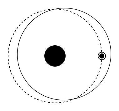A nudged ring particle (blue) and where it would have been on its original circular orbit (hollow). The bar is its radial displacement $y(x)$. The ellipse is exaggerated.

Notice that despite the particle’s angular velocity no longer being constant, its acceleration and deceleration keep the frequency the same.

That frequency influences Saturn’s rings: if the particle’s orbital period is exactly half of Mimas’s, then Mimas’s tug is always maximized at the same point in the particle’s orbit:

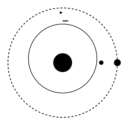A ring particle (blue) at the 2:1 resonance with Mimas (gray). Mimas’s tug (arrow) always lands at the same point in the particle’s orbit. The ellipse is exaggerated.

This phenomenon is called orbital resonance; in the specific case above, an astronomer would (apparently) say that the ring particle is in 2:1 resonance with Mimas.

Let $y(x)$ be the particle’s radial displacement at time $x$, representing the signed length of the green bar in the first animated figure, with time measured so that its natural angular frequency (the rotation of the hollow circle) is $1$.

Then, Mimas’s gravitational pull (represented by the red arrow in the second animated figure) provides a forcing term at that same frequency. Mimas and the particle only rendezvous every other lap, but they always do it at the same point in the swing. Hence the repeating pattern of tugs contains a component at the particle’s own frequency, and that component is all we model:

\[y^{\prime\prime}+y=\cos(x),\qquad y(0)=y^\prime(0)=0 \tag{$E$}\]

The homogeneous solutions are $\cos(x)$ and $\sin(x)$, so the $\cos(x)$ forcing term matches one of the particle’s homogeneous solutions.

Using the exponential formula for $\cos$

\[\cos(x) = \frac{e^{ix} + e^{-ix}}{2}\]

we obtain $\Laplace{\cos(x)}(s)=s/(s^2+1)$. Thus the Laplace transform of $E$ is

\[(s^2+1)Y(s)=\frac{s}{s^2+1},\qquad Y(s)=\frac{s}{(s^2+1)^2}.\]

There are now double poles at both $s=i$ and $s=-i$. Before inverting, we first rearrange to get

\[Y(s)=\frac{1}{4i}\left(\frac{1}{(s-i)^2}-\frac{1}{(s+i)^2}\right),\]

then transform back using $\Laplace{xe^{rx}}(s)=1/(s-r)^2$ and obtain

\[y(x)=\frac{x}{4i}\bigl(e^{ix}-e^{-ix}\bigr)=\frac{x}{2}\sin(x)\]

The forcing stays bounded, but the response has a linearly growing envelope $x/2$ for $x\ge0$.

Interpreting this physically: Mimas keeps pulling on the particle’s radial swings and the effect continues to grow forever. (In reality, nonlinear effects and collisions with other ring particles take over first, but the result is the same.) This means particles can’t settle into quiet circular orbits at that frequency; the frequency is determined by the radius, so Saturn’s B ring ends there.

For comparison, a particle at a different radius has a different orbital period, so Mimas’s tug no longer lines up with its radial swings. Keeping the same zero initial values but changing the forcing frequency to $2$ yields

\[y^{\prime\prime}+y=\cos(2x),\qquad y(0)=y^\prime(0)=0.\]

Now the solution is

\[y(x)=\frac{\cos(x)-\cos(2x)}{3}.\]

The forcing no longer matches a homogeneous solution, and we aren’t forced to add an $x$ term that would cause the solution to explode, hence the above solution is bounded and the particle stays in Saturn’s ring.

Impulses and the Dirac Delta

A force delivered in a very short time can affect a system substantially. Think of striking an object with a hammer, driving over a pothole in a car, or power surging in an electric circuit. The Dirac delta “function” models an instantaneous impulse of unit strength. This extends our discussion beyond continuous forcing; the resulting equations are interpreted using generalized derivatives (explained in the aside below), rather than requiring a classical solution at the instant of the impulse.

First, consider a simpler kind of sudden change: a switch being flipped on and left on.

Definition (Heaviside Step Function)

For $x_0\in\R$, define the Heaviside step function by

\[H(x-x_0) = \begin{cases} 0 & x < x_0 \\ 1 & x > x_0 \end{cases}\]

Conventions disagree on the value of $H(x_0)$; it really depends on what we’re modeling, but we leave it undefined here.

For $x_0\ge0$, integrating directly gives $\Laplace{H(x-x_0)}(s)=e^{-x_0s}/s$. More generally, delaying a function $g$ by $x_0$ and switching it on at $x_0$ multiplies its transform by $e^{-x_0s}$ (substitute $u=x-x_0$):

\[\Laplace{H(x-x_0)g(x-x_0)}(s)=e^{-x_0s}G(s), \qquad G=\Laplace{g}.\]

This shift rule handles forcing that switches on partway through.

The important quantity is the impulse’s total strength, which is actually an integral quantity rather than a function value:

Definition (Dirac Delta “Function”)

For $x_0\in\R$, the Dirac delta $\delta(x-x_0)$ is the unit impulse at $x_0$, characterized by its integrals over intervals:

\[\int_a^b\delta(x-x_0)\,dx = \begin{cases} 1 & a < x_0 < b\\ 0 & x_0 < a \text{ or } b < x_0 \end{cases}\]

Just as with the Heaviside function, conventions disagree on the case where $x_0 = a$ or $x_0 = b$, so we leave it undefined here.

We care about $\delta$ not just because of what it models, but because of the integral equation it produces with other functions:

Theorem (Sifting Property)

Integrating the Dirac delta $\delta$ against any continuous function $\varphi$ picks out its value at $x_0$:

\[\int_{-\infty}^{\infty}\delta(x-x_0)\varphi(x)\,dx=\varphi(x_0).\]

This is the sifting property.

Applying the sifting property to $e^{-sx}$ gives

\[\Laplace{\delta(x-x_0)}(s)=\int_0^\infty e^{-sx}\delta(x-x_0)\,dx=e^{-x_0s},\qquad x_0>0.\]

This is $s$ times $\Laplace{H(x-x_0)}$, exactly what the derivative formula predicts if $\delta(x-x_0)=H^\prime(x-x_0)$. We’ll justify that in the aside below.

Example (Instantaneous Input)

Consider

\[y^\prime+y=\delta(x-x_0),\qquad y(0)=0,\qquad x_0>0.\]

Transforming gives $(s+1)Y(s)=e^{-x_0s}$, so $Y(s)=e^{-x_0s}/(s+1)$. By the shift rule with $g(x)=e^{-x}$, the inverse transform is

\[y(x)=H(x-x_0)e^{-(x-x_0)}=\begin{cases} 0,&0\le x<x_0,\\ e^{-(x-x_0)},&x>x_0. \end{cases}\]

Indeed, directly transforming this expression gives $\int_{x_0}^\infty e^{-sx}e^{-(x-x_0)}\,dx=e^{-x_0s}/(s+1)$ for $\Re(s)>-1$. The impulse produces a jump $y(x_0^+)-y(x_0^-)=1$, after which the solution decays exponentially. Its value at the single instant $x_0$ doesn’t affect its transform or its generalized derivative.

To see why the equation holds, note that the derivative of a piecewise smooth function includes a delta multiplied by the size of each jump. Here the ordinary derivative away from $x_0$ is $-y$, and the unit jump contributes $H^\prime(x-x_0)=\delta(x-x_0)$. This is an example of an impulse response, which models how a linear system responds to a sudden unit input.

What actually is $\delta$?

One might be tempted (as I once was) to experiment with defining the Dirac delta function as the limit of a normal density as the variance $\sigma^2$ tends to zero:

\[\delta(x-x_0)\relatedby{?}{=} \lim_{\sigma\to0^+}\frac{1}{\sigma\sqrt{2\pi}} \exp\left(-\frac{(x-x_0)^2}{2\sigma^2}\right) =\begin{cases} 0,&x\neq x_0,\\ +\infty,&x=x_0. \end{cases}\]

What a fool I was. While this limit does converge pointwise to $0$ for all $x \neq x_0$ as desired, the value at $x_0$ diverging to infinity doesn’t prevent the resulting extended-valued function from having Lebesgue integral $0$ on every interval.

The problem isn’t even that our function would need to take on the value $\infty$; the real problems are

This violates the property of integrals that we should be allowed to “cut out” a single point: if $a < x_0 < b$ and the impulse sits at $x_0$, we should still have
\[\int_{[a, b]} = \int_a^b = \int_a^{x_0} + \int_{x_0}^b = \int_{[a, x_0) \cup (x_0, b]}\]
If we wanted
\[\int_a^b 2\delta(x-x_0) \, dx = \begin{cases} 2, & a < x_0 < b, \\ 0, & \text{otherwise}, \end{cases}\]
would we have to require $2\delta(0) = 2\infty$? That makes no sense; there’s no meaningful way to describe what value this function should take at $x_0$ that allows for different impulse strengths.

The solution is to accept that functions aren’t the only things we can integrate. Consider a function $f$ as having two “parts”:

The “mapping part”, which answers “what value $f(x)$ in the codomain does $x$ get mapped to?”, and
The “integrable part”, which answers a very similar question: “given some nice function $\varphi$, what is $\int f(x)\varphi(x)\,dx$?” An integral over $[a,b]$ is (approximately) the special case where $\varphi$ is $1$ on $[a,b]$ and $0$ elsewhere.

A distribution is only the second part, whether or not it has an associated function to provide the “mapping part”. This is how we can have the Dirac delta, which is just a distribution with no associated function, and also how we can characterize almost-everywhere equality: two functions have the same “integrable part” if and only if their “mapping parts” only disagree rarely (that is, they only disagree on a set of measure zero).

To define distributions clearly, we need to first define what that $\varphi$ thing is:

Definition (Test Function)

A test function on $[a, b]$ is a function $\varphi:\R\to\C$ that’s smooth (infinitely differentiable) on all of $\R$ and $0$ outside $[a, b]$.

Definition (Distribution)

A distribution is a rule $T$ that assigns a number $T(\varphi)\in\C$ to every test function $\varphi$, on any interval, such that

$T$ is linear: $T(c\varphi+\psi)=cT(\varphi)+T(\psi)$ for all test functions $\varphi,\psi$ and constants $c\in\C$, and
$T$ is continuous: if test functions $\varphi_1,\varphi_2,\ldots$ on a common interval $[a,b]$ converge uniformly to $\varphi$, and so do all of their derivatives, then $T(\varphi_n)\to T(\varphi)$.

The first property ensures that the linearity of the integral is respected; the second ensures that limits, solutions to differential equations, and other function-like behavior are preserved.

We usually write $T(\varphi)$ with integral notation:

\[\int T(x)\varphi(x)\,dx\]

even though $T(x)$ might wrongly imply that $T$ assigns values to inputs $x$.

Theorem

A function $g$ that is integrable on every bounded interval gives a distribution through the rule $\varphi\mapsto\int g(x)\varphi(x)\,dx$. For every $x_0\in\R$, the delta’s rule

\[\int_{-\infty}^{\infty}\delta(x-x_0)\varphi(x)\,dx=\varphi(x_0)\]

also gives a distribution, even though no function $g$ produces it.

We differentiate distributions by requiring integration by parts to keep working:

\[\int T^\prime\varphi\,dx=-\int T\varphi^\prime\,dx\]

This is the generalized (or distributional) derivative. (No boundary terms are necessary because test functions vanish outside their interval.) For the unit step $H(x-x_0)$, this gives

\[\int_{-\infty}^{\infty} H^\prime(x-x_0) \varphi(x) \,dx = -\int_{x_0}^\infty \varphi^\prime(x) \, dx = \varphi(x_0)\]

so $H^\prime(x-x_0)=\delta(x-x_0)$. That’s why the jump in our impulse example introduced $\delta$.

As for our Gaussians, they actually do converge to $\delta$ if we integrate before taking the limit:

\[\lim_{\sigma\to0^+}\int_{-\infty}^{\infty} \frac{1}{\sigma\sqrt{2\pi}} \exp\left(-\frac{(x-x_0)^2}{2\sigma^2}\right)\varphi(x)\,dx =\varphi(x_0)\]

for every test function $\varphi$. This is called weak convergence.

Linear Systems of First Order ODEs

Suppose we encounter a system of first-order linear differential equations, where several unknown functions each change at a rate that depends linearly on all of them. These come up all over the place:

Bodies in thermal contact, or sensors in a network, drifting toward a common value
Feedback control, like a motor steering an object back to a target position
Prices adjusting back toward equilibrium after a small market disturbance
Rival nations stockpiling weapons in an arms race

In general, a system of $n$ such equations in $n$ unknown functions $u_1,\ldots,u_n$ looks like

\[\begin{aligned} u_1^\prime&=a_{11}u_1+a_{12}u_2+\cdots+a_{1n}u_n+g_1(x),\\ u_2^\prime&=a_{21}u_1+a_{22}u_2+\cdots+a_{2n}u_n+g_2(x),\\ &\;\;\vdots\\ u_n^\prime&=a_{n1}u_1+a_{n2}u_2+\cdots+a_{nn}u_n+g_n(x) \end{aligned}\]

with constant coefficients $a_{ij}$ and continuous forcing terms $g_i$. Packaging the unknowns, coefficients, and forcing terms into matrices and vectors

\[\mathbf u=\begin{pmatrix}u_1\\\vdots\\u_n\end{pmatrix},\qquad A=\begin{pmatrix}a_{11}&\cdots&a_{1n}\\\vdots&\ddots&\vdots\\a_{n1}&\cdots&a_{nn}\end{pmatrix},\qquad \mathbf g(x)=\begin{pmatrix}g_1(x)\\\vdots\\g_n(x)\end{pmatrix},\]

the whole system becomes a single matrix equation:

\[\mathbf u^\prime=A\mathbf u+\mathbf g(x).\]

By taking eigenvalues of the matrix $A$, we can perform a change of variables that makes the system easier to solve. This is known as the eigenvalue method.

The Eigenvalue Method

Suppose first that $A$ has a basis of eigenvectors, so we can diagonalize it and obtain $A=P\Lambda P^{-1}$ with $\Lambda=\operatorname{diag}(\lambda_1,\ldots,\lambda_n)$. Change variables by setting $\mathbf u=P\mathbf v$, and multiply the system by $P^{-1}$:

\[\mathbf v^\prime=\Lambda\mathbf v+\mathbf h(x), \qquad \mathbf h=P^{-1}\mathbf g\]

Because $\Lambda$ is diagonal, these equations no longer involve each other’s unknown functions, and we obtain

\[v_i^\prime=\lambda_i v_i+h_i(x)\]

We already know how to solve this from our existence proof! Applying that formula to each component gives

\[v_i(x)=e^{\lambda_i(x-x_0)}v_i(x_0) +\int_{x_0}^x e^{\lambda_i(x-t)}h_i(t)\,dt.\]

The exponential term gives the homogeneous solution, and the integral gives a particular solution with initial value zero.

The final step is to revert the change of variables using $\mathbf u=P\mathbf v$ to obtain our solutions $\mathbf u$. If we were given initial conditions, we can plug in $\mathbf v(x_0)=P^{-1}\mathbf u(x_0)$ to obtain the unique solution; otherwise, $v_i(x_0)$ are the free constants for our general solution.

Example (Network Agreement)

Suppose three sensors are connected in a chain, and each sensor $i$ adjusts its reading $u_i$ toward its neighbors’ readings at the same rate. Choosing time units so that this rate is $1$ gives the system

\[\begin{aligned} u_1^\prime&=u_2-u_1,\\ u_2^\prime&=(u_1-u_2)+(u_3-u_2),\\ u_3^\prime&=u_2-u_3. \end{aligned}\]

In matrix form, this is

\[\mathbf u^\prime=A\mathbf u,\qquad A=\begin{pmatrix}-1&1&0\\1&-2&1\\0&1&-1\end{pmatrix}.\]

The eigenvalues of $A$ are $0,-1,-3$, with respective eigenvectors $(1,1,1)^{\mathsf T}$, $(1,0,-1)^{\mathsf T}$, and $(1,-2,1)^{\mathsf T}$. There’s no forcing, so changing variables and solving each $v_i^\prime=\lambda_iv_i$ gives

\[\mathbf u(x)=C_1\begin{pmatrix}1\\1\\1\end{pmatrix} +C_2e^{-x}\begin{pmatrix}1\\0\\-1\end{pmatrix} +C_3e^{-3x}\begin{pmatrix}1\\-2\\1\end{pmatrix}.\]

The sum of the readings stays constant because $u_1^\prime+u_2^\prime+u_3^\prime=0$, so $C_1=(u_1(0)+u_2(0)+u_3(0))/3$. Both disagreement modes decay, so every sensor converges to the average of the initial readings, and the eigenvalues tell us how quickly the disagreements disappear. The same system models three bodies in thermal contact approaching a common temperature.

Example (Market Equilibrium)

A greengrocer’s stall in the Municipal Market of São Paulo. Wilfredor, CC BY-SA 4.0 https://creativecommons.org/licenses/by-sa/4.0, via Wikimedia Commons

Suppose two goods are substitutes, like Coke and Pepsi, Macs and PCs, and so on. Let $u_1$ and $u_2$ be how far their prices are from market equilibrium. Each price falls when it’s above equilibrium, since buyers want less of it, and rises when the other good is more above equilibrium, since buyers switch over. With adjustment rates $2$ and $1$ (in suitable units), this gives

\[\begin{aligned} u_1^\prime&=-2u_1+u_2,\\ u_2^\prime&=u_1-2u_2. \end{aligned}\]

This is a cross-price effect: the price of one good moves the demand of the other. An underpriced good decreases demand for its competitor, and an overpriced good increases demand for its competitor. We can package this system into matrix form as

\[\mathbf u^\prime=A\mathbf u,\qquad A=\begin{pmatrix}-2&1\\1&-2\end{pmatrix}.\]

The eigenvalues of $A$ are $-1$ and $-3$. Because both are negative, the system will eventually settle towards equilibrium. The associated eigenvectors, $(1,1)^{\mathsf T}$ and $(1,-1)^{\mathsf T}$ respectively, tell us how:

\[\mathbf u(x)=C_1e^{-x}\begin{pmatrix}1\\1\end{pmatrix} +C_2e^{-3x}\begin{pmatrix}1\\-1\end{pmatrix},\]

where $C_1=(u_1(0)+u_2(0))/2$ and $C_2=(u_1(0)-u_2(0))/2$.

So, a shared deviation (both prices too high) decays at rate $1$, while a relative deviation (one too high, the other too low) decays three times as fast, because buyers switching between the goods correct the prices from both sides.

We can animate this relationship in phase space, where the coordinates are given by the values of $u_1$ and $u_2$, and the differential equation defines a vector field. Each dot represents one solution to the system, started from a particular initial value pair $(u_1(0), u_2(0))$, moving along the vector field as the system progresses.

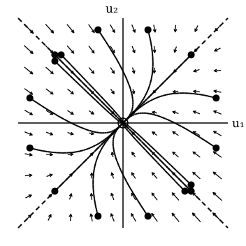Sixteen starting deviations evolving under the market model. The relative deviation (along the rose line) dies out first, so every path bends onto the blue line of shared deviation before settling at equilibrium.

You can imagine a vector field as telling us how water flows, and the dots as leaves that fall onto the water and are carried by the current. An equilibrium is a point where the vector field is zero, so a point there will not move. Our specific system has a sink in the middle (which here corresponds to a local minimum), so all the dots eventually accumulate there. Equilibria tell us a lot about the long-term behavior of the system.

Very roughly speaking, a system is called chaotic if its evolution over time is extremely sensitive to the initial values, even if those initial values are close to each other. Chaos is not a standard topic in these courses because linear systems cannot be chaotic.

Example (Arms Race)

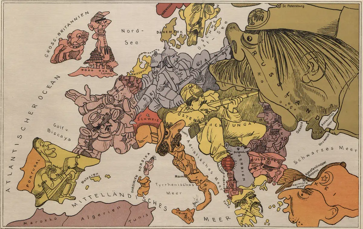Walter Trier’s satirical “Karte von Europa im Jahre 1914” (“Map of Europe in the Year 1914”). Public domain, via Wikimedia Commons

Now suppose two rival nations each stockpile arms in response to the other’s arsenal. This arms race would continue indefinitely, except that the cost to each nation of maintaining their own arsenal slows them down. This is Lewis Fry Richardson’s arms race model.

Let $u_1$ and $u_2$ be how far each nation’s arsenal is above some baseline. If each nation reacts to its rival twice as strongly as it restrains itself, then

\[\begin{aligned} u_1^\prime&=-u_1+2u_2,\\ u_2^\prime&=2u_1-u_2. \end{aligned}\]

This is the market example with the magnitudes of the diagonal and off-diagonal entries swapped:

\[\mathbf u^\prime=A\mathbf u,\qquad A=\begin{pmatrix}-1&2\\2&-1\end{pmatrix}.\]

The eigenvalues of $A$ are $1$ and $-3$, with the same eigenvectors $(1,1)^{\mathsf T}$ and $(1,-1)^{\mathsf T}$ as before, so

\[\mathbf u(x)=C_1e^{x}\begin{pmatrix}1\\1\end{pmatrix} +C_2e^{-3x}\begin{pmatrix}1\\-1\end{pmatrix},\]

with $C_1$ and $C_2$ given by the same formulas as before. A difference between the two arsenals still dies out, but now any shared buildup grows exponentially: a runaway arms race. Making the reaction to the rival stronger than self-restraint turned the eigenvalue $-1$ into $+1$. (As with Saturn’s rings, the linear model eventually stops applying; in reality, budgets — or the will to peace — run out first.)

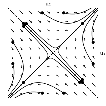The same starting points under the arms race model. Paths still collapse onto the blue line, but now they run away along it. Only starts exactly on the rose line would reach equilibrium; the four just beside it get close before escaping.

The phase space animation shows us that the equilibrium $(0,0)$ is now a saddle point of the system. The rose line has a negative eigenvalue so it collapses everything in towards $0$, and the blue line has a positive eigenvalue so it pushes everything away from $0$. The “knife’s edge” solution demands that our initial conditions start exactly on the rose line.

Now, this would be quite a dour situation, so let’s suppose that at some time $x_0 > 0$ diplomats from the two nations meet and negotiate a détente, with each nation immediately surrendering $k$ units of arms.

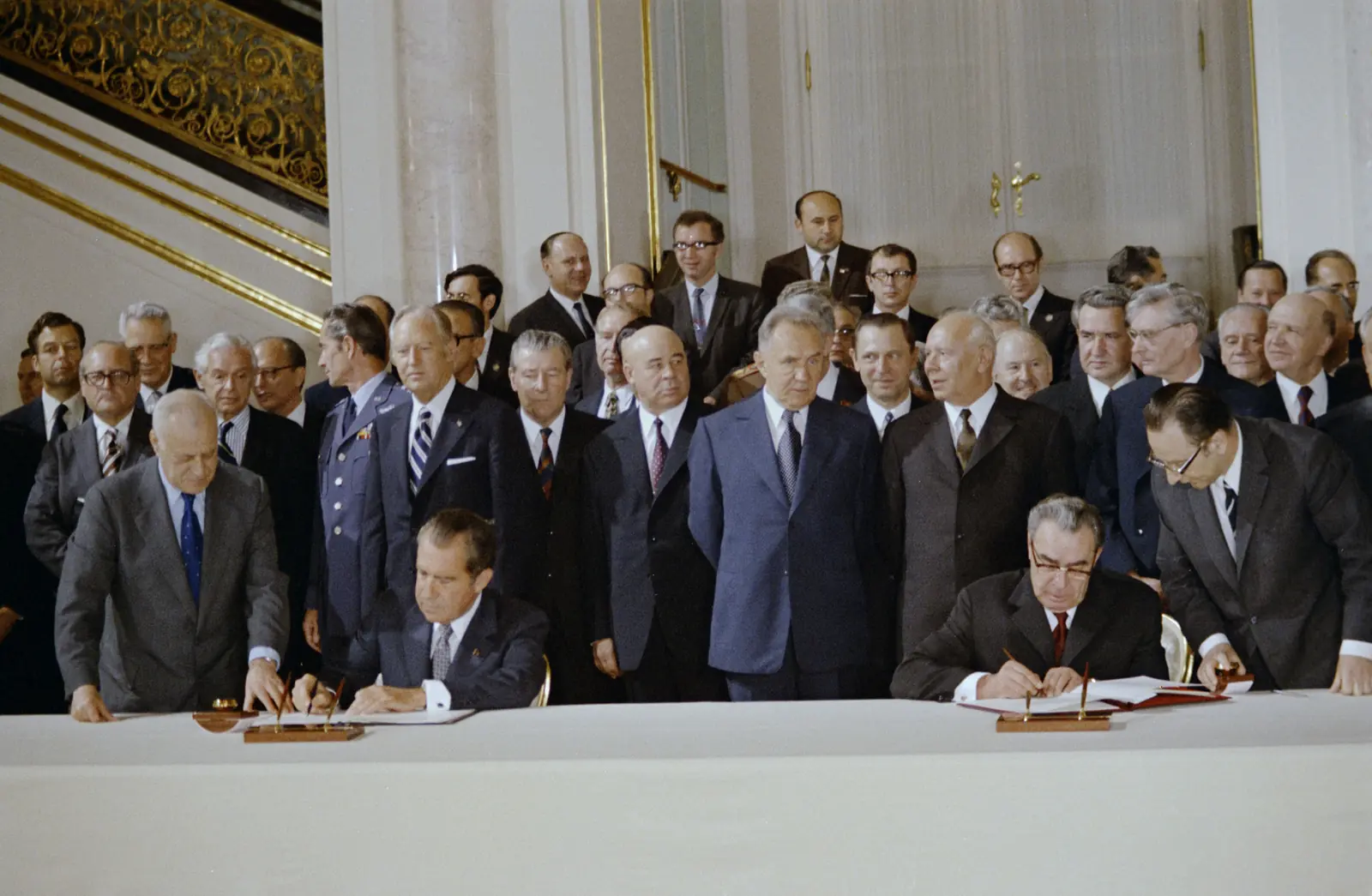Nixon and Brezhnev signing the ABM Treaty and the interim SALT agreement in Moscow on May 26, 1972. White House Photo Office, public domain, via Wikimedia Commons

An instantaneous change like this is an impulse, so the system becomes

\[\mathbf u^\prime=A\mathbf u-k\,\delta(x-x_0)\begin{pmatrix}1\\1\end{pmatrix}.\]

The forcing points along the shared eigenvector $(1,1)^{\mathsf T}$, so after changing variables it only affects the first new equation:

\[v_1^\prime=v_1-k\,\delta(x-x_0),\qquad v_2^\prime=-3v_2.\]

The first-order formula and the sifting property give $v_1(x)=C_1e^x-k\,H(x-x_0)e^{x-x_0}$, so after the negotiation,

\[\mathbf u(x)=\bigl(C_1-ke^{-x_0}\bigr)e^{x}\begin{pmatrix}1\\1\end{pmatrix} +C_2e^{-3x}\begin{pmatrix}1\\-1\end{pmatrix},\qquad x>x_0.\]

The negotiation doesn’t change the eigenvalues, only the coefficient of the runaway mode. Writing $S=C_1e^{x_0}$ for the shared buildup at the moment of signing, there are three possible outcomes when $S > 0$:

If $k<S$, the arms race resumes, just from a lower starting point.
If $k>S$, it reverses into a runaway disarmament.
If $k=S$ exactly, the shared buildup vanishes and both arsenals settle back to the baseline.

That last case is the same knife’s edge as before, since the accord puts the arsenals exactly on the rose line: the baseline is an unstable equilibrium, so any error in the cut eventually reignites one runaway or the other.

Example (Sappho and Her Friend)

Simeon Solomon, Sappho and Erinna in a Garden at Mytilene (1864). Tate Britain, public domain, via Wikimedia Commons

Steven Strogatz famously modeled love affairs with linear systems. Let $u_1$ be the very strong friendliness that the poet Sappho feels for her entirely Platonic friend Erinna, and $u_2$ be Erinna’s friendliness toward Sappho at time $x$, with negative values meaning dislike.

Sappho’s feelings simply follow Erinna’s: the friendlier Erinna is, the faster Sappho warms to her: $u_1^\prime=u_2$.

However, Erinna is more complicated. Her feelings feed on themselves, but Sappho’s friendliness puts her off, and a meddling mutual acquaintance keeps pushing her toward Sappho with some outside influence $f(x)$, so $u_2^\prime=-2u_1+3u_2+f(x)$.

In matrix form, with $\mathbf u=(u_1,u_2)^{\mathsf T}$, this is

\[\mathbf u^\prime=\begin{pmatrix}0&1\\-2&3\end{pmatrix}\mathbf u +\begin{pmatrix}0\\f(x)\end{pmatrix}.\]

This matrix’s eigenvalues are $1$ and $2$, with eigenvectors $(1,1)^{\mathsf T}$ and $(1,2)^{\mathsf T}$. Taking these as the columns of $P$ gives

\[P=\begin{pmatrix}1&1\\1&2\end{pmatrix}, \qquad P^{-1}\mathbf g=\begin{pmatrix}-f\\f\end{pmatrix}\]

The new equations are $v_1^\prime=v_1-f(x)$ and $v_2^\prime=2v_2+f(x)$. Solving these with the first-order formula and reverting our change of variables gives the general solution

\[\mathbf u(x)=C_1e^x\begin{pmatrix}1\\1\end{pmatrix} +C_2e^{2x}\begin{pmatrix}1\\2\end{pmatrix} +\int_{x_0}^x\begin{pmatrix}e^{2(x-t)}-e^{x-t}\\2e^{2(x-t)}-e^{x-t}\end{pmatrix}f(t)\,dt\]

To finish with concrete forcing, suppose the two start as strangers, $\mathbf u(0)=\mathbf 0$ at $x_0=0$, and the acquaintance’s meddling escalates as $f(x)=e^{3x}$. Then $\mathbf v(0)=P^{-1}\mathbf u(0)=\mathbf 0$, and the new equations give

\[\begin{aligned} v_1(x)&=-\int_0^x e^{x-t}e^{3t}\,dt =\frac12e^x-\frac12e^{3x}\\ v_2(x)&=\int_0^x e^{2(x-t)}e^{3t}\,dt =e^{3x}-e^{2x} \end{aligned}\]

which, in the original variables, gives us

\[\mathbf u(x)=P\mathbf v(x) =\begin{pmatrix} \frac12e^x-e^{2x}+\frac12e^{3x}\\ \frac12e^x-2e^{2x}+\frac32e^{3x} \end{pmatrix}\]

In plainer notation, this means our solutions are

\[\begin{aligned} u_1(x)&=\tfrac12e^x-e^{2x}+\tfrac12e^{3x},\\ u_2(x)&=\tfrac12e^x-2e^{2x}+\tfrac32e^{3x}. \end{aligned}\]

Expanding near $x=0$, Erinna warms up first, with $u_2\approx x$, and Sappho follows, with $u_1\approx x^2/2$. Both eigenvalues are positive, so their “friendship” would grow explosively even without the acquaintance’s help: any nonzero homogeneous part grows exponentially.

Since both eigenvalues are positive, our system produces a source at $(0,0)$; going with our water analogy, this would be a water fountain’s pump, or a stream of water falling from above and pushing everything away. (Anything caught exactly in the center — the zero solution — would be pushed equally in all directions, and thus not move anywhere.)

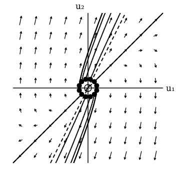The Sappho and Erinna system, without the acquaintance’s meddling. Everything is pushed away from the origin, and the faster-growing rose direction $(1,2)$ (eigenvalue $2$) soon dominates, so paths turn parallel to it unless they start exactly on the blue line $(1,1)$ (eigenvalue $1$).

If our eigenvalues have $\Im \lambda \neq 0$, then we get very fun behavior. Writing the eigenvalues as $\lambda = \alpha \pm \beta i$:

If $\alpha<0$, the origin is a stable spiral. Solutions circle the origin while shrinking like $e^{\alpha x}$, so everything spirals in, like water swirling down a drain.
If $\alpha>0$, the origin is an unstable spiral. Solutions circle the same way while growing like $e^{\alpha x}$, so everything spirals out.
If $\alpha=0$, the origin is a center. Solutions go around closed loops forever, neither pulled in nor pushed out, like a frictionless spring bouncing back and forth.

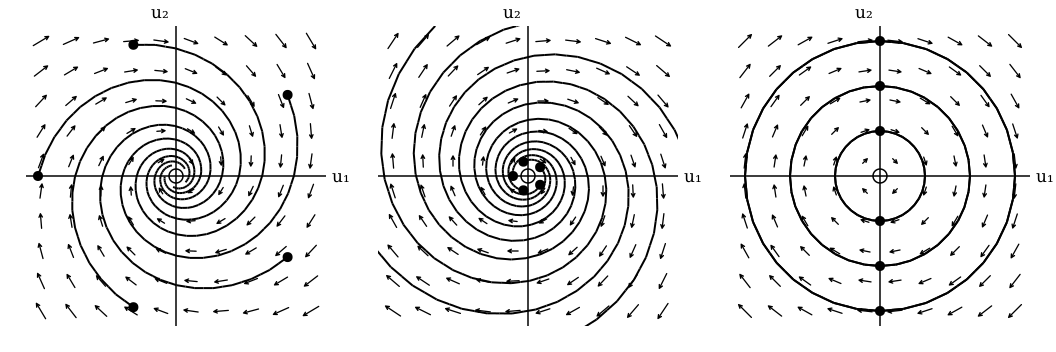Left to right: a stable spiral ($\alpha=-1/4$), an unstable spiral ($\alpha=1/5$), and a center ($\alpha=0$), all with $\beta=1$, which sets how fast solutions turn.

The Matrix Exponential

Anyways, back to our solution method. We can derive a formula for the solution that works for every $A$, although it relies on one function we haven’t introduced yet:

Definition (Matrix Exponential)

Let $A$ be a constant $n\times n$ matrix. Its matrix exponential, sometimes written $e^{Ax}$, is the series

\[\exp(Ax) := \sum_{k=0}^\infty\frac{x^kA^k}{k!}\]

which converges to an $n \times n$ matrix for every $x$.

$A$ being diagonalizable makes this limit substantially easier to compute, but absolute convergence is quite easy to see: define $a = \max_{i,j} \lvert a_{ij} \rvert$, then convergence is immediate by the comparison test in each entry:

\[\lvert \exp(Ax)_{ij} \rvert \leq e^{na\lvert x \rvert} \quad \text{for every } 1 \leq i, j \leq n\]

$\exp(Ax)$ is, of course, the “matrix version” of $e^{\lambda x}$, which acts as the integrating factor in our general formula:

Theorem (Solutions of Constant-Coefficient Linear Systems)

Let $\mathbf g$ be continuous on an open interval $I$, and let $x_0\in I$ and $\mathbf b\in\F^n$. Then the system $\mathbf u^\prime=A\mathbf u+\mathbf g(x)$ has exactly one solution on $I$ with $\mathbf u(x_0)=\mathbf b$, namely

\[\mathbf u(x)=\exp(A(x-x_0))\mathbf b +\int_{x_0}^x \exp(A(x-t))\mathbf g(t)\,dt.\]

Leaving $\mathbf b$ free gives the general solution.

If $A$ is diagonalizable as $A=P\Lambda P^{-1}$ with $\Lambda=\operatorname{diag}(\lambda_1,\ldots,\lambda_n)$, then

\[\exp(Ax)=P\operatorname{diag}(e^{\lambda_1x},\ldots,e^{\lambda_nx})P^{-1}\]

so this formula reproduces the eigenvalue method.

Proof

We first collect three lemmas about the matrix exponential.

It can be differentiated term by term. The same entrywise comparison bounds both the series and its series of derivative terms uniformly for $\lvert x \rvert \leq R$, so by the Weierstrass M-test both converge uniformly there:
\[\sum_{k=0}^\infty \frac{d}{dx} \left( \frac{x^kA^k}{k!} \right) = \sum_{k=1}^\infty\frac{x^{k-1}A^k}{(k-1)!}\]
so
\[\frac{d}{dx}\exp(Ax)=\sum_{k=1}^\infty\frac{x^{k-1}A^k}{(k-1)!}=A\exp(Ax)=\exp(Ax)A\]
Just like the regular exponential, it turns sums into products. Since $Ax_1$ and $Ax_2$ commute, we can apply the binomial theorem to $(Ax_1+Ax_2)^k$. Algebra reveals
\[\exp(A(x_1+x_2))=\exp(Ax_1)\exp(Ax_2)\]
In particular, $\exp(-Ax)\exp(Ax)=\exp(0A)=I$, so $\exp(Ax)$ is always invertible.
We have a convenient expression for its value on diagonalizable $A$. If $A=P\Lambda P^{-1}$, then $A^k=P\Lambda^kP^{-1}$, and
\[\exp(Ax)=P\left(\sum_{k=0}^\infty\frac{x^k\Lambda^k}{k!}\right)P^{-1}=P\operatorname{diag}(e^{\lambda_1x},\ldots,e^{\lambda_nx})P^{-1}\]

Now, we can proceed to existence and uniqueness.

(Existence) Differentiating using lemma 1 and the Leibniz integration rule gives
\[\begin{aligned} \mathbf u^\prime(x) &=A\exp(A(x-x_0))\mathbf b+\exp(0A)\mathbf g(x)+\int_{x_0}^x A\exp(A(x-t))\mathbf g(t)\,dt\\ &=A\exp(A(x-x_0))\mathbf b+A\int_{x_0}^x\exp(A(x-t))\mathbf g(t)\,dt+\mathbf g(x)\\ &=A\left(\exp(A(x-x_0))\mathbf b+\int_{x_0}^x\exp(A(x-t))\mathbf g(t)\,dt\right)+\mathbf g(x)\\ &=A\mathbf u(x)+\mathbf g(x) \end{aligned}\]
At $x=x_0$ the integral vanishes and $\exp(0A)=I$, so $\mathbf u(x_0)=\mathbf b$.
(Uniqueness) If $\mathbf u$ and $\tilde{\mathbf u}$ are two solutions with the same initial value, their difference $\mathbf w=\mathbf u-\tilde{\mathbf u}$ must satisfy $\mathbf w^\prime=A\mathbf w$ and $\mathbf w(x_0)=\mathbf 0$. By lemma 1 and the product rule,
\[\frac{d}{dx}\Bigl(\exp(-A(x-x_0))\mathbf w(x)\Bigr) =\exp(-A(x-x_0))\bigl(\mathbf w^\prime(x)-A\mathbf w(x)\bigr) =\mathbf 0\]
Thus $\exp(-A(x-x_0))\mathbf w(x)$ is constant, equal to its value $\mathbf w(x_0)=\mathbf 0$ at $x_0$. By lemma 2, its inverse is $\exp(A(x-x_0))$; multiplying the two together gives $\mathbf w(x)=\mathbf 0$.

Now, we verify that this reduces to the eigenvalue method. Writing $\mathbf b=P\mathbf v(x_0)$ and using lemma 3,

\[\begin{aligned} \mathbf u(x) &=\underbrace{\exp(A(x-x_0))}_{P\exp(\Lambda(x-x_0))P^{-1}}\,\underbrace{\mathbf b}_{P\mathbf v(x_0)} +\int_{x_0}^x\underbrace{\exp(A(x-t))}_{P\exp(\Lambda(x-t))P^{-1}}\mathbf g(t)\,dt\\ &=P\Bigl(\underbrace{\exp(\Lambda(x-x_0))}_{\operatorname{diag}(e^{\lambda_i(x-x_0)})}\mathbf v(x_0) +\int_{x_0}^x\underbrace{\exp(\Lambda(x-t))}_{\operatorname{diag}(e^{\lambda_i(x-t)})}\underbrace{P^{-1}\mathbf g(t)}_{\mathbf h(t)}\,dt\Bigr)\\ &=P\mathbf v(x) \end{aligned}\]

Since the $i$-th component of the parenthesized vector is

\[e^{\lambda_i(x-x_0)}v_i(x_0)+\int_{x_0}^x e^{\lambda_i(x-t)}h_i(t)\,dt=v_i(x)\]

this is exactly the eigenvalue method’s solution.

If we don’t have an eigenbasis for $A$, then computing $\exp(Ax)$ is a real pain because we can’t just offload the exponent onto a diagonal matrix. Of course, if we don’t have an eigenbasis, Jordan form $A=PJP^{-1}$ is the next best thing. If you’ve encountered Jordan form before, the aside below lays out the general formula; if you haven’t seen the Jordan form, don’t worry, because standard classes only give systems that have diagonalizations.

Computing the Matrix Exponential with Jordan Form

Since $A^k=PJ^kP^{-1}$, the series for the matrix exponential gives $\exp(Ax)=P\exp(Jx)P^{-1}$. Because $J$ is block-diagonal with Jordan blocks $J_1,\ldots,J_\ell$, so is $\exp(Jx)$ with blocks $\exp(J_ix)$.

So we can reduce our problem from exponentiating the Jordan matrix $J$ down to exponentiating Jordan blocks $J_i$. Let $J_i=\lambda I+N$ denote a block of size $m$, where $N$ has ones immediately above the diagonal and zeros elsewhere:

\[J_i=\begin{pmatrix}\lambda&1&&\\&\lambda&\ddots&\\&&\ddots&1\\&&&\lambda\end{pmatrix} =\lambda I+\underbrace{\begin{pmatrix}0&1&&\\&0&\ddots&\\&&\ddots&1\\&&&0\end{pmatrix}}_{N}.\]

Each power of $N$ pushes its ones one further up the diagonal, so $N^m=0$. Since $\lambda I$ commutes with $N$, $\exp(J_ix)=e^{\lambda x}\exp(Nx)$, and the series for $\exp(Nx)$ stops after $m$ terms:

\[\begin{array}{r@{}c} N={}&\begin{pmatrix}0&1&0&\cdots&0\\&0&1&\ddots&\vdots\\&&\ddots&\ddots&0\\&&&0&1\\&&&&0\end{pmatrix}\\[1ex] N^2={}&\begin{pmatrix}0&0&1&\cdots&0\\&0&0&\ddots&\vdots\\&&\ddots&\ddots&1\\&&&0&0\\&&&&0\end{pmatrix}\\[1ex] &\vdots\\[1ex] N^{m-1}={}&\begin{pmatrix}0&0&0&\cdots&1\\&0&0&\cdots&0\\&&\ddots&\ddots&\vdots\\&&&0&0\\&&&&0\end{pmatrix}\\[1ex] N^m={}&0 \end{array}\]

So after $k \geq m$, the matrix settles, and we get our formula for the Jordan block:

\[\exp(J_ix)=e^{\lambda x}\sum_{k=0}^{m-1}\frac{x^kN^k}{k!} =e^{\lambda x}\begin{pmatrix}1&x&\frac{x^2}{2}&\cdots&\frac{x^{m-1}}{(m-1)!}\\&1&x&\ddots&\vdots\\&&\ddots&\ddots&\frac{x^2}{2}\\&&&1&x\\&&&&1\end{pmatrix}\]

which gives us the value of $\exp$ on $J$:

\[\exp(Jx)=\begin{pmatrix}\exp(J_1x)&&\\&\ddots&\\&&\exp(J_\ell x)\end{pmatrix}\]

Plugging $\exp(Ax)=P\exp(Jx)P^{-1}$ into the theorem’s formula solves any constant-coefficient system, with or without forcing. Thus our final, most general formula is

\[\mathbf u(x)=P\exp(J(x-x_0))P^{-1}\mathbf b+\int_{x_0}^xP\exp(J(x-t))P^{-1}\mathbf g(t)\,dt\]

The powers of $x$ in $\exp(Nx)$ provide the functions $x^k/k!$, and the whole expression $\exp(J_ix)$ turns them into the basis functions $e^{\lambda x}x^k/k!$.¹ We last saw this when discussing resonance, and that’s the underlying cause of our missing eigenbasis. For a forcing term $e^{rx}\mathbf w$, the scalar factor $z = e^{rx}$ is itself a solution of $z^\prime = rz$, so we can fold it into the system as one more unknown, giving a homogeneous system with the block matrix

\[\begin{pmatrix}A&\mathbf w\\0&r\end{pmatrix}\]

If $r$ is already an eigenvalue of $A$ and $\mathbf w$ has a nonzero component along $r$’s eigenvector, this larger matrix has too few eigenvectors for $r$, and its Jordan block produces the extra factor of $x$.

Example

Consider

\[A=\begin{pmatrix}1&1\\-1&3\end{pmatrix}.\]

Its characteristic polynomial is $(s-2)^2$, but its eigenspace is only $\Span\set{(1,1)^{\mathsf T}}$, so we don’t have an eigenbasis. Set $\mathbf w_1=(1,1)^{\mathsf T}$ and solve $(A-2I)\mathbf w_2=\mathbf w_1$. One choice is $\mathbf w_2=(0,1)^{\mathsf T}$. Thus

\[P=\begin{pmatrix}1&0\\1&1\end{pmatrix},\qquad J=P^{-1}AP=\begin{pmatrix}2&1\\0&2\end{pmatrix}.\]

This is a single Jordan block of size $2$, so $N^2=0$ and

\[\exp(Jx)=e^{2x}(I+xN)=e^{2x}\begin{pmatrix}1&x\\0&1\end{pmatrix}.\]

Writing $\mathbf v(0)=P^{-1}\mathbf u(0)=(C_1,C_2)^{\mathsf T}$, the solution of $\mathbf u^\prime=A\mathbf u$ is

\[\begin{aligned} \mathbf u(x)&=P\exp(Jx)P^{-1}\mathbf u(0)\\ &=Pe^{2x}\begin{pmatrix}C_1+C_2x\\C_2\end{pmatrix}\\ &=e^{2x}\begin{pmatrix}C_1+C_2x\\C_1+C_2x+C_2\end{pmatrix} \end{aligned}\]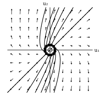

A degenerate node. The repeated eigenvalue $2$ has only one eigenvector, $(1,1)$, so the blue line is the only straight path, and every other path turns toward its direction as the $C_2xe^{2x}$ term takes over.

Higher Order Equations as Systems

So far, this section hasn’t said a word about the $n$-th order equations we started with. The twist is that they were systems all along. We can reduce an $n$-th order linear ODE to a system of first-order equations. Start with

\[c_ny^{(n)}+\cdots+c_1y^\prime+c_0y=f(x), \qquad c_n\neq 0\]

Collect the unknown function and its first $n-1$ derivatives into a vector:

\[\mathbf u(x)=\bigl(y(x),y^\prime(x),\ldots,y^{(n-1)}(x)\bigr)^{\mathsf T}\]

The first $n-1$ entries differentiate to the next entry, and the original equation tells us the derivative of the last entry. Thus

\[\mathbf u^\prime=A\mathbf u+\mathbf g(x)\]

For $n=1$, this is simply $A=(-c_0/c_1)$ and $\mathbf g=(f/c_1)$. For $n\ge 2$,

\[A=\begin{pmatrix} 0&1&\cdots&0\\ \vdots&\ddots&\ddots&\vdots\\ 0&\cdots&0&1\\ -c_0/c_n&-c_1/c_n&\cdots&-c_{n-1}/c_n \end{pmatrix}, \qquad \mathbf g(x)=\begin{pmatrix}0\\\vdots\\0\\f(x)/c_n\end{pmatrix}\]

In either case, the initial conditions become $\mathbf u(x_0)=(b_0,\ldots,b_{n-1})^{\mathsf T}$.

This provides a path to reduce linear systems of higher order ODEs (including “systems” with only one equation) down to linear systems of first order ODEs. If we obtained this system from a single higher-order equation, we recover its general solution $y$ by taking the first component of $\mathbf u$. In the diagonalizable case, writing $C_i=v_i(x_0)$, this is

\[y(x)=\sum_{i=1}^n P_{1i}\left( C_i e^{\lambda_i(x-x_0)} +\int_{x_0}^x e^{\lambda_i(x-t)}h_i(t)\,dt \right)\]

Example

The earlier Sappho/Erinna system with eigenvalues $1$ and $2$ comes from $y^{\prime\prime}-3y^\prime+2y=f(x)$. Its first component gives

\[y(x)=C_1e^x+C_2e^{2x} +\int_{x_0}^x\bigl(e^{2(x-t)}-e^{x-t}\bigr)f(t)\,dt\]

For $f(x)=e^{3x}$ and zero initial values at $x=0$, the first component of our evaluated system solution is exactly the solution we obtained using the Laplace transform.

Solution Sets

Now that we know how to find solutions, we should probably try to characterize them. You may have noticed that our uniqueness result required specifying initial conditions

\[y^{(k)}(x_0)=b_k, \qquad 0 \le k<n\]

on $y$ and its derivatives, representing data at a single point. However, without them, we end up with a whole space of solutions: recall that we got solutions like $C_1e^x$ or $C_1\sin(x) + C_2\cos(x)$, where each coefficient $C_i$ was free. The functions multiplied by these free coefficients form a basis for that space, and these initial conditions pluck out a unique solution from it.

These solution sets look kinda like vector spaces; the coefficients $C_i$ look like the coefficients for basis vectors. However, those extra terms like $x$ have fixed coefficients, and when the forcing term is not identically zero, our space doesn’t contain the “zero vector” $y(x) = 0$.

What is actually going on here?

What we’re really looking at is something called an affine space, which is roughly “a vector space plus a vector”:

Definition (Affine Space)

Let $W$ be any $\F$-vector space. Given any vector subspace $V \subseteq W$ and any translation vector (or base point) $a \in W$, the translate

\[\mathcal{A} = V + a := \setbuild{v + a}{v \in V}\]

is called an affine subspace of $W$, and comes equipped with the following properties:

(Differences lie in the underlying vector space) If $p,q \in \mathcal{A}$, then $p-q \in V$. Conversely, if $p \in \mathcal{A}$ and $v \in V$, then $p + v \in \mathcal{A}$.
(Any point can serve as the translation vector) For every $a \in \mathcal{A}$, we have $\mathcal{A} = V + a$.
(Affine combinations stay in the space) If $a_1,\ldots,a_k \in \mathcal{A}$ and $\lambda_1,\ldots,\lambda_k \in \F$ satisfy $\lambda_1+\cdots+\lambda_k=1$, then
\[\lambda_1a_1 + \cdots + \lambda_ka_k \in \mathcal{A}\]
In particular, the entire line through any two distinct points of $\mathcal{A}$ lies in $\mathcal{A}$. Arbitrary linear combinations need not lie in $\mathcal{A}$.
(The translate is a vector subspace exactly when it contains zero) Equivalently, $\mathcal{A}$ is a vector subspace of $W$ if and only if $a \in V$, in which case $\mathcal{A}=V$.

Furthermore, if $V$ is finite-dimensional with basis $v_1,\ldots,v_n$, then every $p \in \mathcal{A}$ has a unique expression

\[p = a + c_1v_1 + \cdots + c_nv_n, \qquad c_1,\ldots,c_n \in \F\]

We call $n$ the dimension of $\mathcal{A}$.

So the general solution $y$ to a linear ordinary differential equation with constant coefficients takes the form

\[y(x) = \underbrace{C_1\beta_1(x) + \cdots + C_n\beta_n(x)}_{\text{an element of } V} + \underbrace{y_p(x)}_a\]

where the $\beta_i$ are basis functions for $V$ and $y_p$ arises because of the forcing term $f(x)$. If we could just delete that forcing term, we’d end up with the equation

\[c_ny^{(n)} + \cdots + c_1y^\prime + c_0y = 0 \tag{$E_h$}\]

which we called $E$’s associated homogeneous differential equation. We write $\mathcal{S}(E)$ for the set of solutions of an equation $E$.

Example

For $E: y^\prime=y-x$, the associated homogeneous equation is $E_h:y^\prime=y$. Its solution space is $\mathcal S(E_h)=\Span\set{e^x}$.

Example

For $E:y^{\prime\prime}=y-x^2$, the associated homogeneous equation is $E_h:y^{\prime\prime}=y$. Its solution space is $\mathcal S(E_h)=\Span\set{e^x,e^{-x}}$.

In general, if $E_h$ is any homogeneous linear ODE of order $n$, then its solution set $\mathcal{S}(E_h)$ forms a vector space:

Theorem (Solution Sets of Homogeneous Linear ODEs)

Let $E_h$ be a homogeneous linear ordinary differential equation of order $n$ with constant coefficients in $\F$:

\[c_ny^{(n)}+\cdots+c_1y^\prime+c_0y=0, \quad c_n \neq 0 \tag{$E_h$}\]

Then the solution set $\mathcal{S}(E_h)$ of $E_h$ on $I$ forms an $n$-dimensional $\F$-vector space.

Proof

We have two tasks: to show that $\mathcal{S}(E)$ is a vector space, and to show that it’s $n$-dimensional.

($\mathbf{\mathcal{S}(E)}$ is a Vector Space): First, we must prove that $\mathcal{S}(E)$ forms a vector space. We can do that using the more general “subspace trick”, where we show that a set (here, $\mathcal{S}(E)$) forms a vector space by showing that it is a subset of some ambient vector space $W$, that it contains the zero vector in $W$, and that it is closed under linear combinations.
We can choose $C^n(I, \F)$, the $\F$-vector space of all $n$-times continuously differentiable functions on the interval $I$. You should be able to easily verify that this is a vector space under pointwise addition with the zero vector given by the zero function.
Clearly $\mathcal{S}(E) \subset C^n(I, \F)$; now, we must only check the two criteria; we can do this most conveniently by introducing the linear differential operator associated with $E$, $L_E$ (not to be confused with the Laplace transform $\mathscr{L}$!), that sends $y$ to the left-hand side of $E$:
\[L_E[y] := c_ny^{(n)}+\cdots+c_1y^\prime+c_0y\]
so $\mathcal{S}(E)$ is the set of all $y$ with $L_E[y]=0$. Differentiation is linear, so $L_E$ is too: for any functions $u,v$ and scalars $a,b\in\F$,
\[L_E[au+bv]=aL_E[u]+bL_E[v]\]
Now the criteria are almost trivial to verify:
- (Zero Vector): The zero vector of $C^n(I, \F)$ is the zero function, and $L_E[0] = 0$, so it’s a member of $\mathcal{S}(E)$.
- (Closure Under Linear Combinations): If $L_E[u]=L_E[v]=0$ then $L_E[au+bv]=0$, so $au + bv \in \mathcal S(E)$.
That makes it a subspace of $C^n(I, \F)$, hence a vector space.
($\mathbf{\dim \mathcal{S}(E) = n}$): Fix a point $x_0 \in I$ and define a map $T$ that sends each solution to its initial values:
\[\begin{aligned} T:\mathcal S(E)&\longrightarrow\F^n\\ y&\longmapsto\bigl(y(x_0),y^\prime(x_0),\ldots,y^{(n-1)}(x_0)\bigr). \end{aligned}\]
$T$ is linear because differentiation and evaluation at $x_0$ are linear, and the composition of linear operators is linear. Now, we want to prove it’s a bijection, which is given by our theorem on the existence and uniqueness of solutions to $E$:
- (Surjectivity) Existence says that for every tuple in $\F^n$, there is some solution with those initial values, so $T$ is surjective.
- (Injectivity) Uniqueness says each tuple can be matched to only one solution, so $T$ is injective.
Linear bijections are isomorphisms, so $T$ is an isomorphism of vector spaces. The codomain $\F^n$ is $n$-dimensional, so $\mathcal S(E)$ must be as well.

Going back to our inhomogeneous linear ODE $E$, the solution set $\mathcal{S}(E_h)$ to its associated homogeneous differential equation $E_h$ is exactly the vector space $V$ that we wanted to construct our affine space $\mathcal{S}(E)$ from! But what will we use for $a$?

Recall that a particular solution $y_p$ is any solution to the inhomogeneous equation $E$. Subtracting $y_p$ from any solution of $E$ gives a solution of $E_h$, and adding $y_p$ to any solution of $E_h$ gives a solution of $E$. Thus $\mathcal{S}(E)=\mathcal{S}(E_h)+y_p$; property 2 in our affine spaces discussion tells us that we don’t care which one. We can find it, as well as the basis vectors $\beta_i$ of $\mathcal{S}(E_h)$, using the techniques above.

Okay, so putting this all together:

Theorem (Solution Sets of Linear ODEs)

Suppose that we have an $n$-th order linear ordinary differential equation with constant coefficients in $\F$, where $c_n \neq 0$:

\[c_ny^{(n)} + \cdots + c_1y^\prime + c_0y = f(x) \tag{$E$}\]

If the forcing term $f$ is not identically zero, then the set of solutions $\mathcal{S}(E)$ is an affine space given by

\[\mathcal{S}(E) = \mathcal{S}(E_h) + y_p\]

where $\mathcal{S}(E_h)$ is the $n$-dimensional vector space of solutions to the associated homogeneous differential equation

\[c_ny^{(n)} + \cdots + c_1y^\prime + c_0y = 0 \tag{$E_h$}\]

and $y_p$ is any solution to $E$. If $f(x) = 0$ identically, then the solution set is simply the vector space $\mathcal{S}(E_h)$.

So finding a general solution for $E$ amounts to finding a particular solution $y_p$ and a basis of functions $\beta_1(x), \beta_2(x), \ldots, \beta_n(x)$ for $\mathcal{S}(E_h)$, and every solution $y_h$ to the homogeneous equation can be expressed uniquely in that basis:

\[y_h(x) = C_1\beta_1(x) + \cdots + C_n\beta_n(x)\]

Once we’ve found a $y_p$, initial conditions $y^{(k)}(x_0)=b_k$ for $0 \le k<n$ uniquely specify these coefficients $C_i$ as solutions to the system of linear equations

\[\begin{aligned} C_1\beta_1(x_0)+\cdots+C_n\beta_n(x_0)&=b_0-y_p(x_0),\\ C_1\beta_1^\prime(x_0)+\cdots+C_n\beta_n^\prime(x_0)&=b_1-y_p^\prime(x_0),\\ &\vdots\\ C_1\beta_1^{(n-1)}(x_0)+\cdots+C_n\beta_n^{(n-1)}(x_0)&=b_{n-1}-y_p^{(n-1)}(x_0). \end{aligned} \tag{$C_E$}\]

This linear system $C_E$ is guaranteed to have exactly one solution $(C_1,\ldots,C_n)$ by the existence and uniqueness of solutions to ordinary differential equations. With those coefficients, basis functions, and $y_p$ in hand, we can map this solution $y_h$ to a solution $y$ by the affine translation

\[\begin{aligned} \tau_{y_p}:\mathcal{S}(E_h)& \longrightarrow \mathcal{S}(E)\\ y_h& \mapsto y_h+y_p \end{aligned}\]

giving a solution $y$ in $\mathcal{S}(E)$ to the full, inhomogeneous equation with the prescribed initial conditions.

This dovetails nicely with linear algebra: the basis guarantees that our coefficients $C_i$ represent $y_h = y-y_p$ uniquely.

What’s $W$?

There are two useful choices for $W$:

The smallest possible ambient space: $W = \mathcal{S}(E_h) + \Span\set{y_p}$. If the forcing term is not identically zero, $y_p \not \in \mathcal{S}(E_h)$, so a basis of $\mathcal{S}(E_h)$ can be extended to a basis of $W$ by adjoining $y_p$. Since $\dim \mathcal{S}(E_h) = n$, we get $\dim W = n+1$.
A function space: for an ODE of order $n$ on an interval $I$, we can let $W$ be the function space $C^n(I, \F)$ of all $n$-times continuously differentiable functions from $I$ to $\F$. We saw this before in our proof that $\mathcal{S}(E_h)$ forms a vector space.

$W = \mathcal{S}(E_h) + \Span\set{y_p}$ is easy enough to construct and very easy to think about after we know $y_p$, but the larger function space is available before we know $y_p$. Of course, studying this second space is a serious digression from a first course in ODEs; my point in presenting $C^n$ is to whet our appetite for deeper studies in analysis.

Why would we ever expect this to work?

This becomes pretty easy to see if we develop a little bit of the theory of operators. An operator is a fancy term for a higher-order function: one that takes in functions and spits out functions. The derivative $D$ is one such operator:

\[\begin{aligned} D: C^n(I, \R)& \longrightarrow C^{n-1}(I, \R)\\ y& \mapsto y^\prime \end{aligned} \qquad (n\ge1)\]

where $C^n(I, \R)$ is the space of all functions $f: I \to \R$ that are $n$-times continuously differentiable on the interval $I$. (If we’re considering the space of infinitely differentiable functions $C^{\infty}(I, \R)$ or $C^{\infty}(I, \C)$, then $D$ is a linear map from each of these spaces to itself. A linear map like that is called a linear endomorphism.)

The derivative is only the simplest in a large family of operators, called differential operators. If you read the proof that solution spaces to homogeneous linear equations form a vector space, you’ll recall the linear differential operator associated with $E$, the operator $L_E$ that sends $y$ to the linear combination of it and its derivatives contained in $E$:

\[L_E[y] := c_ny^{(n)}+\cdots+c_1y^\prime+c_0y\]

So the original equation and its associated homogeneous equation can be expressed as

\[E: L_E[y] = f, \qquad E_h: L_E[y] = 0\]

For constant coefficients, it’s conventional to write $L_E=p(D)$, where $p(s)=c_ns^n+\cdots+c_1s+c_0$ is the characteristic polynomial of $E$.

Exponentials are eigenfunctions (that is, eigenvectors which also just so happen to be functions) of $D$:

\[D(e^{\lambda x})=\lambda e^{\lambda x}, \qquad L_E[e^{\lambda x}]=p(\lambda)e^{\lambda x}\]

Thus every root $\lambda$ of $p$ gives a homogeneous solution $e^{\lambda x}$. (The $\lambda$s are doing double duty: they are both eigenvalues and polynomial roots!) A root of multiplicity $m$ contributes the functions $e^{\lambda x},xe^{\lambda x},\ldots,x^{m-1}e^{\lambda x}$. Together, these give a basis of the homogeneous solution space.

Proof (Why do these functions form a basis?)

First, we show that each of these $n$ functions is a solution, then that they’re linearly independent.

(Solutions): Write $m_r$ for the multiplicity of each distinct root $r$, and let $D-r$ denote the operator
\[(D-r)[y] = y^\prime - ry.\]
Then by the product rule,
\[(D-r)\bigl[e^{rx}q(x)\bigr]=e^{rx}q^\prime(x)\]
for any polynomial $q$, so $(D-r)^{m_r}$ annihilates (sends to $0$) $x^ke^{rx}$ for $k<m_r$:
\[(D-r)^{m_r}\left[x^ke^{rx}\right] = 0\]
The factors of $p(D)$ commute, so $p(D)=g(D)(D-r)^{m_r}$ for some polynomial $g$, and
\[p(D)\left[x^ke^{rx}\right]=g(D)\Bigl[(D-r)^{m_r}\left[x^ke^{rx}\right]\Bigr]=0.\]
So each of these functions is a member of $\mathcal S(E_h)$.
(Linear Independence): Write the distinct roots as $r_1,\ldots,r_\ell$ with multiplicities $m_1,\ldots,m_\ell$, and suppose $\sum_{j=1}^\ell e^{r_jx}q_j(x)=0$ with $\deg q_j<m_j$. Fix an index $i$ and apply $\prod_{j\neq i}(D-r_j)^{m_j}$, which annihilates every term except the $i$-th and leaves
\[e^{r_ix}\prod_{j\neq i}(D+r_i-r_j)^{m_j}q_i(x)=0.\]
Each factor $D+(r_i-r_j)$ with $j\neq i$ preserves the degree of a nonzero polynomial, so $q_i=0$. Since $i$ was arbitrary, every $q_i=0$.

Because there are $\sum_j m_j= n$ of these functions $x^ke^{rx}$ in our $n$-dimensional solution space $\mathcal S(E_h)$ and they’re all linearly independent, they span and are thus a basis for the space. This basis is over $\C$; the real replacements are described above.

The matrix constructed from the scalar equation has characteristic polynomial $p(s)/c_n$, so its eigenvalues are exactly these roots; its Jordan blocks account for the powers of $x$.

This provides yet another connection between an ODE and its characteristic polynomial: the linear operator is that characteristic polynomial in $D$. That tedious method that we gave in the proof that solutions to linear ODEs exist way back in the existence and uniqueness section is called “factoring the operator” for this reason.

This also provides one reason to suspect that the Laplace transform and the eigenvalue method are more closely related than they appear. In fact, the solutions to the homogeneous linear equation $E_h$ are the eigenfunctions of $L_E$ with eigenvalue $0$, together with the zero function (in other words, $L_E$’s kernel). We’ll discuss the role of eigenfunctions shortly in the final aside of the article.

What about non-constant coefficients?

The solution-space theory still works if the coefficients and forcing term are continuous on $I$ and $c_n(x)\neq 0$ everywhere on $I$:

\[c_n(x)y^{(n)} + \cdots + c_1(x)y^\prime + c_0(x)y = 0\] \[c_n(x)y^{(n)} + \cdots + c_1(x)y^\prime + c_0(x)y = f(x)\]

Initial conditions still determine a unique solution on $I$, the homogeneous solution space $\mathcal{S}(E_h)$ is still a vector space of dimension $n$, and the inhomogeneous solution set is an affine space given by translating $\mathcal{S}(E_h)$ by any particular solution. The differential operator is still linear, and we can still rewrite the equation as a first-order system, now with a matrix $A(x)$.

Unfortunately, the solution methods do break down somewhat. There’s no single constant-coefficient characteristic polynomial to solve, and diagonalizing $A(x)$ separately at each point generally doesn’t separate the equations: if $\mathbf u=P(x)\mathbf v$, differentiating introduces an extra term $P^\prime(x)\mathbf v$.

That said, if the non-constant coefficients are polynomials, the Laplace transform still works, but just yields another ODE in $s$ (which is hopefully easier to solve). The eigenvalue method works in special cases if we can prove $A(x_0)A(x_1) = A(x_1)A(x_0)$ for any $(x_0, x_1)$ or if $A$ is periodic, but these two cases require additional elbow grease.

At some point, we run into something like differential Galois theory. Just like (algebraic) Galois theory tells us that some polynomials cannot be solved in radicals, differential Galois theory tells us which linear differential equations cannot be solved in exponentials and integrals. “Most” linear ODEs with non-constant coefficients don’t admit those solutions, much less closed-form solutions. I’m told power series, Frobenius series, or variation of parameters are powerful methods, but (in my opinion) the most practical advice for solving differential equations is to either

Home in on the particular equations that you’re likely to encounter in real life, or
Just use numerical methods (which are very robust and broadly applicable).

Conclusion

I hope that you have enjoyed our journey through the theory of linear ordinary differential equations; I have tried to make it more interesting and theoretically satisfying than my undergraduate course.

This isn’t a very high bar to clear. The typical undergraduate course spends weeks drilling a single technique to solve equations, laboriously producing pages’ worth of calculations per equation, with such exciting applications as mixing liquids in a tank or solving Hooke’s law for a bouncing spring.

The reward at the end of each unit was learning a marginally less annoying technique, rendering the previous one entirely obsolete. By the end of the course, students were expected to have memorized Laplace transforms; tests packed so many questions into such a short period of time that any students who used the guess-and-check method (that they had practiced for weeks!) would not finish.

This semester-long trolling campaign is especially heinous in the 21st century, when every single equation in the entire curriculum (plus many, many more beyond) can be solved with eight lines of MATLAB:

MATLAB

syms y(x)

equation = ...;

% general solution
solution = dsolve(equation);

% initial_values = [b_0, b_1, ..., b_{n-1}]
conditions = sym([]);
for k = 0:numel(initial_values)-1
    conditions(end+1) = subs(diff(y,x,k), x, x0) == initial_values(k+1);
end
solution = dsolve(equation, conditions);

Python

import sympy as sp

x = sp.symbols("x")
y = sp.Function("y")

equation = sp.Eq(...)

# general solution
solution = sp.dsolve(equation, y(x))

# initial_values = [b_0, b_1, ..., b_{n-1}]
ics = {y(x).diff(x, k).subs(x, x0): value for k, value in enumerate(initial_values)}
solution = sp.dsolve(equation, y(x), ics=ics)

If you think the theory that we developed might have been interesting enough to offset the tedium, I am sorry to report that almost all of it is hidden for the engineers’ sake: no proofs are ever provided, the term “affine” is never even spoken once, and we certainly never hear anything about linear differential operators or function spaces, no matter how valuable and efficient they would be. My own course didn’t discuss phase space at all. You would be forgiven for not recognizing that the Laplace transform and the eigenvalue method are actually the same!

Yes, they are the same

Both of our methods are fundamentally about rewriting the derivative operation $D$ as multiplication by some value:

\[\text{Laplace transform:}\quad \Laplace{Dy}(s)=s\Laplace{y}(s)-y(0) \tag{$L$}\] \[\text{Eigenvalue method:}\quad D\mathbf u=A\mathbf u \tag{$M$}\]

The Laplace transform turns $D$ into multiplication by the number $s$ at the cost of managing an additional initial-value term. The eigenvalue method collects a homogeneous solution and its derivatives into $\mathbf u=(y,y^\prime,\ldots,y^{(n-1)})^{\mathsf T}$, which turns $D$ into multiplication by the matrix $A$; diagonalizing $A$ then turns it into multiplication by the numbers $\lambda_i$. Both work because exponentials are the eigenfunctions of the derivative:

\[De^{sx}=se^{sx}\]

Here, the eigenvalue is $s$. Hence writing a function in terms of exponentials turns differentiation into multiplication, because we’re acting on an eigenbasis.

In fact, the two methods produce literally the same formulas. Applying equation $L$ to each entry of equation $M$ gives $s\mathbf U-\mathbf u(0)=A\mathbf U$, where $\mathbf U=\Laplace{\mathbf u}$. Diagonalizing $A=P\Lambda P^{-1}$, with eigenvectors $\mathbf p_i$ as the columns of $P$ and $\mathbf v(0)=P^{-1}\mathbf u(0)$, then gives

\[\begin{alignedat}{3} \mathbf U(s)&=(sI-A)^{-1}\mathbf u(0)&&\quad=P(sI-\Lambda)^{-1}P^{-1}\mathbf u(0)&&\quad=\sum_{i=1}^n\frac{v_i(0)}{s-\lambda_i}\,\mathbf p_i\\ \mathbf u(x)&=\exp(Ax)\mathbf u(0)&&\quad=P\exp(\Lambda x)P^{-1}\mathbf u(0)&&\quad=\sum_{i=1}^n v_i(0)\,e^{\lambda_ix}\,\mathbf p_i \end{alignedat}\]

Each expression in the top row is the Laplace transform of the one below it. On the right, the partial-fraction decomposition of $\mathbf U$ is, term by term, the expansion of $\mathbf u$ in the eigenvectors of $A$: each pole $s=\lambda_i$ is an eigenvalue of $A$.

The only difference between them is how much each method diagonalizes. The Laplace transform diagonalizes $D$ on (roughly) all functions, so every value of $s$ shows up, and forcing terms and initial values are handled in the same algebraic step. The eigenvalue method only diagonalizes $D$ on the $n$-dimensional space of homogeneous solutions, where the only exponentials left are the $e^{\lambda_ix}$; that turns the problem into finite-dimensional linear algebra, but forcing has to be handled separately with an integral.

When $A$ has no eigenbasis, both methods respond in the same way: a Jordan block of size $k$ corresponds to a pole of order $k$, and both produce the same $x^je^{\lambda x}$ terms.

So really, we only learn one method that’s actually useful.

If you read the proofs or asides (I hope you did 🙂) you’ll have noticed most of them just tumble right out of the theory of linear differential operators. Had I broken from convention and taught this material that way, I could have saved us both a lot of time.

But I stuck to the standard presentation to make clear just how threadbare these courses really are, and to convince as many students as possible to not waste their time taking them. They’re little more than a certificate that an engineer knows what an ordinary differential equation even is in the first place so they don’t get confused when their boss gives them something to plug into WolframAlpha.

One MIT professor, Gian-Carlo Rota, was press-ganged into teaching undergraduate differential equations for years because he wrote a textbook on the subject. He regretted it so much that he ultimately presented a talk where he called these ODE courses “hopelessly obsolete”:

Some time ago, I received a review copy of Cauchy’s introductory course in differential equations… But it was also a surprise to discover how little the content of the course has changed since Cauchy. Practically the only change has been the introduction of systems, which have made their way down the ladder since my days as a graduate student.
As I read Cauchy’s textbook, I realized how much of the material we now teach is obsolete. The order of presentation of the outworn topics has not been altered. The most preposterous items are found at the beginning, when the text (any text) will list a number of disconnected tricks that are passed off as useful, such as exact equations, integrating factors, homogeneous differential equations, and similarly preposterous techniques. Since it is rare – to put it gently – to find a differential equation of this kind ever occurring in engineering practice, the exercises provided along with these topics are of limited scope: as a matter of fact, the same sets of exercises have been coming down the pike with little change since Euler. Lecturers in the course, most of whom are unaware of any applications of differential equations beyond those given in elementary texts, scrupulously follow the traditional order of the material, as if it were a religious rite; their ignorance of the broader theory of ordinary differential equations makes them sensitive to change.
Why is it that no one has undertaken the task of cleaning the Augean stables of elementary differential equations? I will hazard an answer: for the same reason why we see so little change anywhere today, whether in society, in politics, or in science. Vested interests dominate every nook and cranny of our society, even the society of mathematicians. A revamped elementary differential equations course would require Professor Neanderthal at Oshkosh College to learn the subject anew. The fatuous, expensive, multi-colored textbooks that are now cornering the market would be forced out of print. New textbooks would have to be written. We know what an effort goes into writing a textbook, and how negatively such an effort is rewarded. No clear-headed young mathematician will risk ruining his or her career by writing such a book, as I did.
The sophomore course in differential equations will never be reformed. It will die of natural death, and it will be replaced by several shorter courses that will deal with realistic aspects of differential equations. It is to be hoped that these new courses will be taught by mathematicians rather than by engineers: the budget of any mathematics department is entirely dependent on the number of engineering students enrolled in our elementary courses. Were it not for these courses, which engineers generously defer to mathematicians, our mathematics departments would be doomed to extinction.

Rota said this in 1997. Thirty years later, nothing has changed.

Footnotes

When $\lambda=-1$, you may recognize this as the probability mass function $\Pr\left[\text{Poisson}(x) = k \right]$, or the probability density $f(x)$ of the $\text{Gamma}(k+1,1) = \text{Erlang}(k+1,1)$ distribution. These functions are obtained by exponentiating Jordan blocks! ↩

math

This post is licensed under CC BY 4.0 by the author.

What’s a Differential Equation?

Existence and Uniqueness of Solutions

Solving Equations

The Laplace Transform

Real Solutions from Complex Solutions

Resonance

Impulses and the Dirac Delta

Linear Systems of First Order ODEs

The Eigenvalue Method

The Matrix Exponential

Higher Order Equations as Systems

Solution Sets

Conclusion

Footnotes

Trending Topics