What is the Fourier Transform?

There is geometry in the humming of the strings.
— Pythagoras

The Fourier transform is one of the most profound discoveries in mathematics, which spurred the formalization of mathematical analysis, the field that contains calculus, differential equations, and more. The Fourier transform also underpins sonar, radar, radio, Wi-Fi, Bluetooth, song-finding software like Shazam, and heavily influenced the .jpeg and .mp3 file formats.

The Fourier transform is also something that can be studied at many levels of complexity, with each layer introducing increasingly profound concepts that apply widely in math. Stein and Shakarchi’s four-book Princeton Lectures in Analysis series, a staple of undergraduate and graduate curricula alike, are premised on this idea: each book introduces a new sub-field of analysis (Fourier analysis, complex analysis, measure theory, and functional analysis) to provide more insight into the Fourier transform. The geometric Langlands correspondence, a major conjecture at the very cutting edge of mathematics which was only finally proven in 2024, is itself a deeper level on which to understand the Fourier transform. (Specifically, the Fourier-Mukai transform.)

It’s a rite of passage for engineers and mathematicians to burn the midnight oil trying to grasp what the Fourier transform actually does and what its results even mean. I hope to introduce the major concepts (at least as far as Stein and Shakarchi) in a deep and precise way that doesn’t require reading four volumes of math textbooks.

This article should be accessible to anyone comfortable with single-variable calculus and linear algebra, and just explains what the Fourier transform is, where it comes from, and how to interpret it. This article provides the foundation for two further articles, which are independent: one article on a finer point (whether the Fourier transform is a change of basis or not) that introduces some higher-level linear algebra, and another on real-world algorithms that implement the Fourier transform which is targeted at computer scientists.

Taylor Series

If you don’t need a refresher on Taylor series, I encourage you to jump to the next section.

Introducing Taylor Series

Transcendental functions $y = \sin(x)$ are extremely mysterious. We do have a rule to calculate what its values are, but most people don’t care to break out their ruler and compass and measure the side lengths of triangles. Similarly for $y = \ln(x)$; its value is the solution to $e^y = x$ for positive real $x$, but a naive solution is simply trial and error unless you want to integrate

\[\ln(a) = \int_1^a \frac{1}{x} \, dx\]

But I myself am a bit of an algebra guy; I would prefer to work with polynomials rather than do integrals. Thankfully, Taylor series have us covered.

In general, suppose we have a function $f$ like $\sin(x)$ or $\ln(x)$ that we can differentiate infinitely many times. (This should cover basically every function you see in calculus class.) We can try building a polynomial that approximates $f(x)$ accurately. For now, instead of approximating the entire function, let’s just approximate $f(x)$ at a specific point, $a$, and see what happens. Let’s call our first estimate $T_1(x)$, and just require

\[T_1(a) = f(a)\]

Boom. Great stuff. But this approximation is pretty terrible, all things considered. Where can we go from here?

Well, the nice thing about differentiable functions is that they’re “locally linear”: if you zoom in really far, then the function looks like a straight line, so let’s make a second approximation $T_2$ with:

\[\begin{aligned} T_2(a) &= f(a)\\ T_2^\prime(a) &= f^\prime (a) \end{aligned}\]

This is satisfied by the equation for the tangent line at $a$, which we remember from calculus: \(T_2 = f(a) + f^\prime(a)(x-a)\)

In the case of $f(x) = \sin(x)$ and $a = 0$, this simplifies to $\sin(x) \approx T_2(x) = x$. Engineers use this approximation all the time, but having seen some of the other math engineers do, I don’t trust their judgement all that much. Let’s see if we can do better and try to capture the curvature of $f(x)$ as well. From physics class, we know second derivatives capture the idea of acceleration. Let’s add that in:

\[\begin{aligned} T_3(a) &= f(a)\\ T_3^\prime(a) &= f^\prime (a)\\ T_3^{\prime\prime}(a) &= f^{\prime \prime} (a)\\ \end{aligned}\]

So this is about the point where approximations tend to be pretty nice (or at least, not atrocious) in the real world. Of course, this approximation is only good when we stick “close” to $a$: in other words, $T_n$ is a local approximation, kind of the same way that the derivative is a local approximation of a function’s rate of change.

If you try this method yourself on a “reasonably nice” function $f$ (for example, $\sin(x)$ or $\ln(x)$), you’ll see the area around $a$ where $T_n$ is accurate seems to grow as $n$ gets larger. If we want to extrapolate out our strategy for building $T_n$ for any $n \in \N$, we just need two criteria:

1. $T_n^{(m)}(a) = f^{(m)}(a)$ for all $0 \leq m \leq n$.
2. $T_n$ is a polynomial of degree $n$.

These two requirements together are actually strict enough to require $T_n$ to always look a specific way:

\[T_n(x) = f(a) + f^\prime(a)(x-a) + \frac{f^{\prime\prime}(a)}{2}(x - a)^2 + \cdots = \sum_{m=0}^n \frac{f^{(m)}(a)}{m!}(x-a)^m\]

You can verify for yourself that this formula works: if you take the $k$th derivative, you’ll notice that the zeros of the polynomial terms $(x-a)^m$ ensures that the term with the $f^{(m)}/m!$ coefficient will be zero — basically, the other derivatives’ values won’t interfere with $T_n^{(k)}$’s values. We include that $m!$ term on the bottom so that repeated differentiation won’t disturb $f^{(m)}(a)$ as we multiply by $m$, $m-1$, $\ldots$ when applying the power rule.

So basically, we end up with a function whose first $n$ derivatives at $a$ exactly match the first $n$ derivatives of $f$ at $a$. As we do this, the region where $T_n$ provides a good approximation for $a$ often continues to expand; obviously, there are cases like $1/x$ and $a = 1$ where the asymptote kinda “gets in the way” and prevents us from getting a good approximation for the negative numbers, but for some “well behaved” functions we just get a better and better approximation the closer to $a$ we get.

Taylor polynomials of sin(x) centered at 0

We’re obliged to ask: what happens if we take $\lim_{n \to \infty} T_n$? Does that region where we get a good approximation extend to all of $\R$, making for an “infinitely accurate approximation”?

Taylor’s theorem says yes!

Theorem (Taylor’s Theorem) Let $f$ be $(n+1)$-times differentiable on an open interval containing $a$ and $x$. Then

\[f(x) = T_n(x) + R_n(x), \qquad R_n(x) = \frac{f^{(n+1)}(c)}{(n+1)!}(x-a)^{n+1}\]

for some $c$ between $a$ and $x$.

$R_n$ is the term “remaining” between our polynomial $T_n$ and $f$. If $R_n(x) \to 0$ as $n \to \infty$ for $x$ near $a$, then $T_n(x) \to f(x)$: the infinite Taylor series converges right back to the function it came from. Functions with this property get their own name:

Definition (Analytic) Let $f: \R \to \C$ be infinitely differentiable. We call $f$ analytic if, around every point $a$, the Taylor series of $f$ centered at $a$ converges to $f$ on some open interval containing $a$:

\[\lim_{n \to \infty} T_n(x) = f(x) \quad \text{for all } x \text{ near } a\]

Note that convergence is only required locally: $1/(1+x^2)$ is analytic, even though its Taylor series at $0$ only converges on $(-1, 1)$.

Analytic functions are some of the nicest functions to work with because Taylor series are so well-behaved and give us so much information. For example, they give us a convenient way to approximate transcendental functions like $\sin(x)$ and give us a hard upper limit on our error. In addition, if we’ve proven some basic facts about how to manipulate Taylor series and how Taylor series behave with the imaginary unit $i$ (defined such that $i^2 = -1$), we can immediately derive Euler's formula

\[\cos(x) + i\sin(x) = e^{ix}\]

from directly comparing their Taylor series.

Fourier Series

Periodic Functions and Decompositions

Taylor series are not the only way to represent a function as a series. Joseph Fourier (1768-1830) was working on a differential equation called the heat equation, which is closely related to equations that model the stock market (the Black-Scholes equation), Brownian motion (the Fokker-Planck equation), and quantum mechanics (the Schrödinger equation). In one spatial dimension, the heat equation models the diffusion of heat along a rod:

\[\frac{\partial f}{\partial t} = \frac{\partial^2 f}{\partial x^2}\]

Fourier realized that if the rod had finite length $L$, the solution could be considered periodic with period $L$. Recall what it means for a function to be periodic:

Definition (Periodic) We say a function $f:\R \to \C$ is periodic if there exists a positive real number $p$ such that $f(x) = f(x + p)$ for all $x$. We call such a number a period of $f$.

If even one such $p$ exists, then there are infinitely many: $f(x) = f(x + p) = f(x + 2p) = f(x+ 3p)$ and so on. If $f$ is periodic, continuous, and non-constant, then there is a smallest $p$, which we define to be the period.

The most obvious examples of periodic functions are, of course, sine waves, which have period $2\pi$. Working with sine waves, Fourier discovered solutions to the heat equation could be found and expressed most conveniently not as a Taylor series whose terms are the polynomials $1, x, x^2, x^3, \ldots$, but rather a series of sine and cosine waves. These series are called Fourier series.

Many functions permit a Fourier series; for example, consider the square wave function with period $p = 2\pi$:

\[f(x) = \begin{cases} \hphantom{-}1 & x \in \left(2k\pi, (2k + 1)\pi\right) \\ -1 & x \in \left( (2k+1) \pi, (2k + 2)\pi \right) \end{cases} \qquad \text{for every integer } k.\]

Fourier deduced that this function can be represented as:

\[f(x) = \frac{4}{\pi}\sum_{k=0}^{\infty} \frac{\sin\left((2k+1)x\right)}{2k+1} = \frac{4}{\pi}\left(\sin(x) + \frac{\sin(3x)}{3} + \frac{\sin(5x)}{5} + \cdots\right)\]

Partial sums $S_n(x)$ of the square wave's Fourier series, more odd harmonics at a time.

Two things are worth watching in the figure. First, at each jump ($x = 0, \pi, 2\pi, \ldots$) every partial sum passes through $0$, the average of the plateau values $\pm 1$ on either side. Second, the little overshoot that appears on either side of each jump doesn’t shrink as more terms are added; it holds steady at about $9\%$ of the jump’s height and simply squeezes into a narrower and narrower sliver around the discontinuity. This is Gibbs' phenomenon: the partial sums still converge to $f$ in $L^2$ (the overshoot’s shrinking width means it vanishes in the limit), just not uniformly near a jump.

Deriving Fourier Series

The intuition for finding these coefficients is kind of like reading off individual coordinates for a vector. Suppose I’m working in $\R^2$ with the standard basis

\[\begin{bmatrix} 1 \\ 0 \end{bmatrix}, \begin{bmatrix} 0 \\ 1 \end{bmatrix}\]

and I wanted a matrix formula to grab an entry out of a vector $\vec v$ in that space. Well, if you want the first coordinate, just take the dot product against the first basis vector, and if you want the second coordinate, take the dot product against the second basis vector:

\[\begin{bmatrix} 1 \\ 0 \end{bmatrix} \cdot \begin{bmatrix} v_1 \\ v_2 \end{bmatrix} = v_1 \qquad \begin{bmatrix} 0 \\ 1 \end{bmatrix} \cdot \begin{bmatrix} v_1 \\ v_2 \end{bmatrix} = v_2\]

There’s a very high level way (that I cover in Is the Fourier Transform a Change of Basis?) in which the integral formulas

\[\frac{2}{p}\int_0^p f(x)\cos\left(2\pi\frac{n}{p}x\right)dx \qquad \frac{2}{p}\int_0^p f(x)\sin\left(2\pi\frac{n}{p}x\right)dx\]

are doing that exact thing: the integral is the dot product in a vector space of functions. Doing these integrals for each $n$ pulls out the corresponding coefficients for each of the “basis vectors” (terms) in the “linear combination” (Fourier series). Here, we split the coefficients up into even (cosine) and odd (sine). Putting this all together, we get the coefficient formulas below:

Definition (Fourier Series for Periodic Functions) Let $f : \R \to \C$ be square-integrable with period $p$. Then the Fourier series of $f$ is

\[f(x) = a_0 + \sum_{n=1}^{\infty}\left(a_n \cos\left(2\pi \frac{n}{p} x\right) + b_n \sin\left(2\pi\frac{n}{p} x\right) \right)\]

where the coefficients are given by

\[\begin{aligned} a_0 &= \frac{1}{p}\int_0^p f(x)\,dx \\ a_n &= \frac{2}{p}\int_0^p f(x)\cos\left(2\pi\frac{n}{p}x\right)dx \\ b_n &= \frac{2}{p}\int_0^p f(x)\sin\left(2\pi\frac{n}{p}x\right)dx \end{aligned}\]

Worked Example: The Square Wave

Plugging $f$ into the coefficient formulas with $p = 2\pi$, $a_0 = 0$ (the plateaus have equal and opposite area) and every $a_n = 0$ too, since $\int_0^\pi \cos(nx)\,dx$ and $\int_\pi^{2\pi} \cos(nx)\,dx$ both vanish for integer $n$. The sine coefficients do the actual work:

\[b_n = \frac{1}{\pi}\left(\int_0^\pi \sin(nx)\,dx - \int_\pi^{2\pi} \sin(nx)\,dx\right) = \frac{2\left(1 - (-1)^n\right)}{n\pi} = \begin{cases} \dfrac{4}{n\pi} & n \text{ odd} \\ 0 & n \text{ even} \end{cases}\]

Only the odd harmonics survive, each shrinking like $1/n$, so

\[f(x) = \frac{4}{\pi}\sum_{k=0}^{\infty} \frac{\sin\left((2k+1)x\right)}{2k+1} = \frac{4}{\pi}\left(\sin(x) + \frac{\sin(3x)}{3} + \frac{\sin(5x)}{5} + \cdots\right)\]

Intuition for Fourier Series

A Fourier series pulls our function apart into its corresponding frequencies the same way that a Taylor series pulls our function apart into polynomial terms. It’s helpful to provide a visual, where a function that doesn’t appear to have any connection to sine waves (on this interval) is actually the sum of four of them:

A signal pulled apart into four sine waves.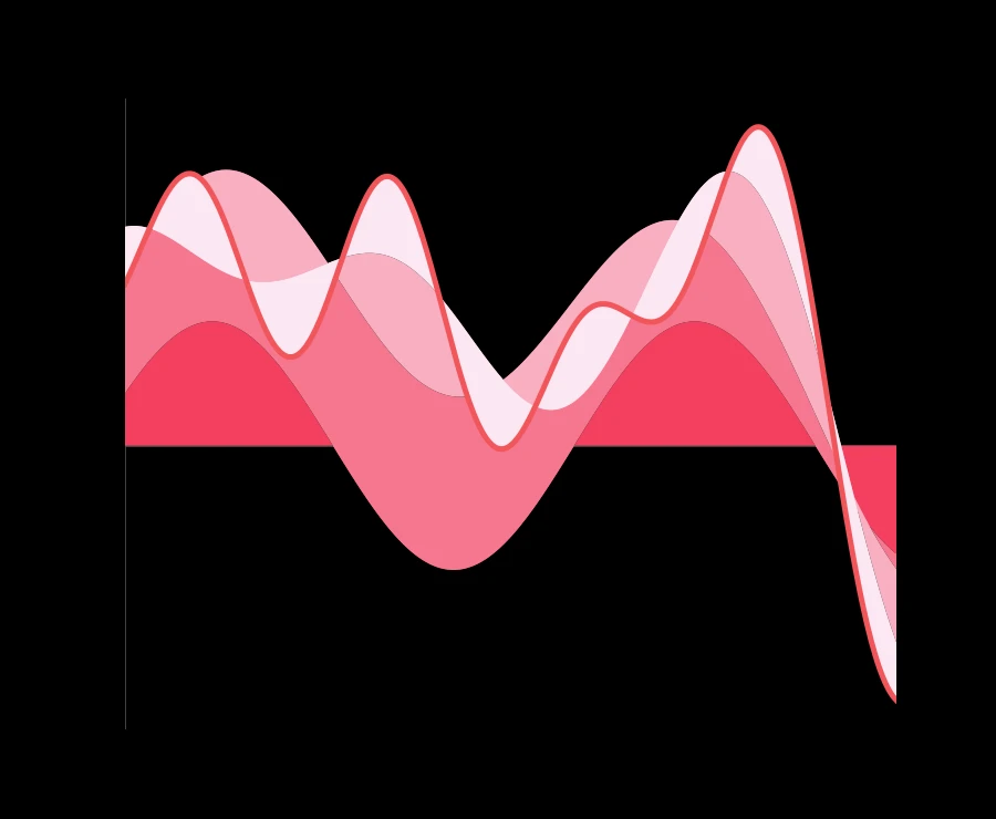

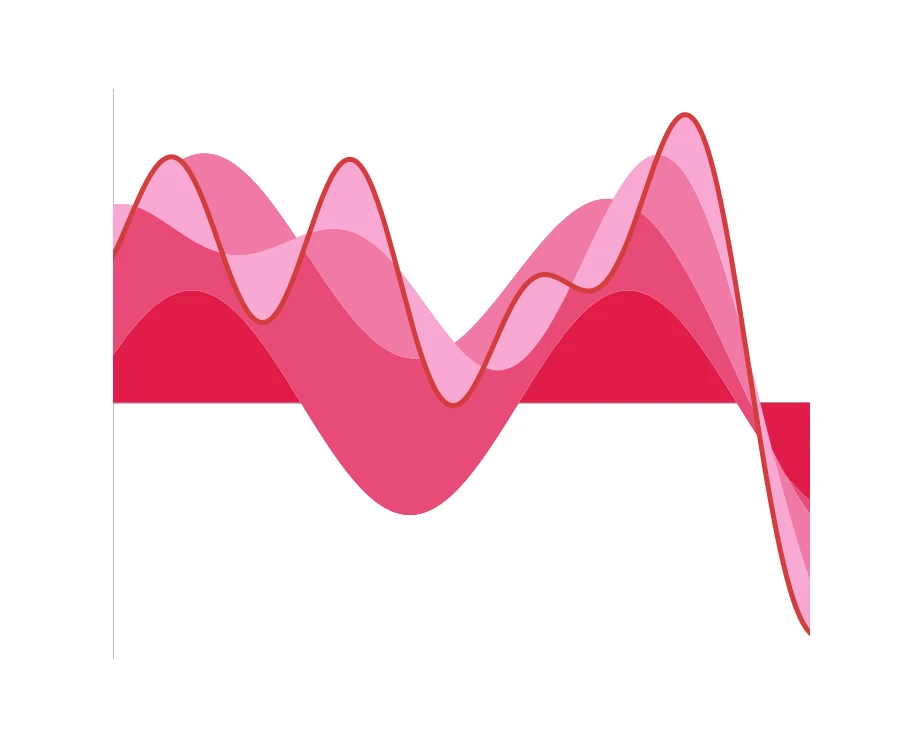The same signal shown as a stacked area chart.

I also often think about this idea like stacked area charts, the kind of which you might find in Our World In Data. I want to be crystal clear this isn’t a direct analogy, but I think of it very roughly like switching between a stacked area chart ($f$) and a line chart ($\hat f$), where the line charts are the individual frequencies. This is also why we take the Fourier transform: if we’re reading a raw signal, we would only see the total value — in this case, CO₂ emissions — rather than the contributions. It’s the same data, just two different ways to view it.

A stacked area chart decomposes into regional lines. Data: Our World in Data, CO2 and Greenhouse Gas Emissions (CC BY).

Which Functions Have Fourier Series?

Just like how analytic functions have criteria (infinitely differentiable with convergent Taylor series), there are two criteria for a function to have a Fourier series; the first is that the function must be periodic, as we’ve already discussed. The second is that it must be absolutely integrable on $[0, p)$:

Definition (Absolute Integrability) A function $f: \R \to \C$ is called absolutely integrable on the interval $[a, b]$ if the integral of its absolute value converges:

\[\int_a^b |f(x)| \, dx < \infty\]

The space of all such functions on $[a, b]$ is denoted $L^1[a,b]$.

Absolute integrability looks a little weird, but it prevents a lot of weird and nasty behavior: the integral of $f$ can never be undefined or diverge to $\pm \infty$; this is enough to ensure the coefficient integrals converge. Absolute integrability also exorcises other pathological behavior we’d prefer to avoid, like any asymptotes not being “too bad”.

However, you may recall from our earlier discussion on Taylor series that if we have a function $f$ that’s infinitely differentiable, that’s enough to define Taylor series, but not enough to guarantee that the Taylor series actually converges to $f$. We have a similar situation here; $f$ being absolutely integrable ensures that its Fourier coefficients are well-defined, but doesn’t ensure that the resulting Fourier series converges back to $f$. For that, we need square integrability on $[0, p)$:

Definition (Square Integrability) A function $f: \R \to \C$ is called square-integrable on $[a, b]$ if the integral of its squared absolute value converges:

\[\int_a^b |f(x)|^2 \, dx < \infty\]

The space of all such functions on $[a, b]$ is denoted $L^2[a,b]$.

If we’re working on a bounded interval like $[a, b]$, every square-integrable function is also absolutely integrable, so $L^2[a,b] \subseteq L^1[a,b]$, and it’s enough to just require $f$ to be in $L^2$.

Typically, the only other requirement we might add in is piecewise differentiability, because then the series converges to $f(x)$ wherever $f$ is continuous, and to the average of the left and right limits at a jump discontinuity.

Precise Notes on Convergence

There are a couple senses in which the Fourier series converge. First, in the $L^2$ sense that the integral of the squared error between the Fourier series and $f$ over the period $p$ goes to $0$.

Second, the series converges pointwise almost everywhere thanks to Carleson’s theorem.

However, almost everywhere convergence still allows for convergence to fail on a set of measure zero, and sets of measure zero can have infinitely many points and be quite poorly behaved; we’d probably prefer something that doesn’t look like the Dirichlet function. Besides piecewise differentiability, we can just insist that $f$ have bounded variation or be Hölder continuous on an interval to guarantee it converges everywhere on that interval.

Why Fourier Series Are Worth Studying

Fourier series are compelling and provocative for several reasons.

1. They’re indispensable for solving partial differential equations, which are differential equations that involve partial derivatives with respect to different variables. Joseph Fourier was particularly interested in the heat equation, which in one spatial dimension can be written as:

   \[\frac{\partial f}{\partial t} = \frac{\partial^2 f}{\partial x^2}\]

   This represents, for example, how fast heat diffuses along a rod. Additional dimensions can be added to model sheet metal or other situations. It’s easiest to find solutions to this equation by assuming that the function $f$ that solves the equation has a Fourier series representation; this turns out to not only yield a solution, but the only solution. This equation is tied to the Black-Scholes equation in finance and the Schrödinger equation in physics.

2. $\sin(x)$ is an odd function, and cosine is an even function. These classes of function are so named because their products behave just like sums of even and odd integers: the product of two even functions is even, the product of two odd functions is also even, and the product of an even and an odd function is odd. Sums are even more predictable: a sum of even functions is always even, and a sum of odd functions is always odd. However, using Fourier series, the odd function $f(x) = x$ can be expressed as a series of even functions:

   \[x = \frac{\pi}{2} - \frac{4}{\pi}\left(\frac{\cos(x)}{1^2} + \frac{\cos(3x)}{3^2} + \frac{\cos(5x)}{5^2} + \cdots\right) \quad \text{for } 0 \le x \le \pi\]

   This was scandalous in the early 1800s; mathematicians debated if such a counterintuitive result indicated that Fourier’s promising and powerful theory was flawed. This challenge to the intuition of the time motivated Augustin-Louis Cauchy (1789-1857) and Karl Weierstrass (1815-1897) to put calculus, which had been quite wishy-washy and underdeveloped by modern standards, on a much more rigorous ground. Their campaign resulted in the extraordinarily large field now known as mathematical analysis.

3. Sound waves and electrical signals are periodic and are obvious candidates to be represented as Fourier series. This is how Fourier analysis allows us to decode messages over Wi-Fi, radio, or audio.

The Fourier Transform

Non-periodic Functions

The sound made by a single handclap, a five-minute song over the radio, or a lightning strike aren’t (or at least, don’t have to be) periodic, yet they clearly have data that we should expect the Fourier transform to be able to capture; how can we extend the Fourier transform to non-periodic functions?

Fourier bridged this gap by cleverly treating one-off signals (non-periodic functions) as the limiting case of a periodic signal: we simply take the limit as $p$ goes to infinity, pushing the repetitions “infinitely far away” until only a single copy of the signal is left behind. (This means we require absolute integrability on all of $\R$, but plenty of functions satisfy this requirement.)

To see what happens to the Fourier series in the limit, let’s rewrite it using Euler’s formula from earlier. Substituting

\[\cos(\theta) = \frac{e^{i\theta}+e^{-i\theta}}{2} \qquad \sin(\theta) = \frac{e^{i\theta}-e^{-i\theta}}{2}i\]

into the definition above and collecting terms, the pair of sums over cosines and sines collapses into a single sum of complex exponentials, now indexed over all integers $n \in \Z$:

\[f(x) = \sum_{n=-\infty}^{\infty} c_n \, e^{2\pi i \frac{n}{p} x}, \qquad c_n = \frac{1}{p}\int_0^p f(x)\, e^{-2\pi i \frac{n}{p} x}\, dx\]

(For real-valued $f$, $c_n$ and $c_{-n}$ turn out to be complex conjugates of each other, so their imaginary parts cancel out and we recover $a_n$ and $b_n$.)

Every term in this sum oscillates at one of the frequencies $\xi_n = n/p$, spaced $1/p$ apart. As $p \to \infty$, that spacing shrinks to $0$, and the available frequencies go from a sparse, evenly-spaced lattice to a set that eventually “fills up” every real number. The point is, all this stuff converges nicely because we demanded that $f$ be absolutely integrable which ensures our formulas handle the case where $f$ isn’t periodic.

Deriving the Fourier Transform

There’s a catch. The coefficient $c_n$ has a factor of $1/p$ sitting in front of its integral, so each individual $c_n$ is being squeezed toward $0$ right along with the frequency spacing. To get something that survives the limit, consider $p \times c_n$ instead, which cancels that factor:

\[p \times c_n = \int_{-p/2}^{p/2} f(x)\, e^{-2\pi i \frac{n}{p}x}\, dx\]

Hold the frequency $\xi = n/p$ fixed while $p \to \infty$ (the integration window grows to cover the whole real line right along with it), and this converges to a genuine function of a continuous frequency variable $\xi$:

\[\hat{f}(\xi) = \int_{-\infty}^{\infty} f(x)\, e^{-2\pi i \xi x}\, dx\]

$\hat{f}$ is called the Fourier transform of $f$, also written $\Fourier{f}$: instead of a discrete list of coefficients $\ldots, c_{-1}, c_0, c_1, \ldots$, one per harmonic, we get a single continuous function $\hat f(\xi)$ that reports how much of frequency $\xi$ is “present” in $f$, for every real $\xi$.

Think of the function $e^{-2\pi i \xi x}$, called the kernel of the transform, as a detector tuned to one pure tone. For a fixed $\xi$, the integral holds that detector against the entire signal at once and measures how well $f$ lines up with it: wherever $f$ oscillates in step with the tone, the products reinforce each other, and wherever it doesn’t, they cancel. The louder that tone is in $f$, the larger $\lvert \hat f(\xi) \rvert$ comes out. Changing $\xi$ is like turning a radio dial, which tunes the detector to a new frequency and takes the reading again. (We’ll explore this intuition more below.)

Deriving the Inverse Fourier Transform

We can use the same limiting trick to go in the reverse direction and reconstruct $f(x)$ from $\hat f(\xi)$. Since $c_n = \hat f(\xi_n)/p$ and consecutive frequencies are spaced $\Delta \xi = 1/p$ apart, the Fourier series can be rewritten as

\[f(x) = \sum_{n=-\infty}^{\infty} \hat f(\xi_n)\, e^{2\pi i \xi_n x} \, \Delta \xi\]

which is exactly a Riemann sum, in the variable $\xi$, with mesh width $\Delta \xi$. As $p \to \infty$, that mesh shrinks to $0$ and the sum converges to an integral:

\[f(x) = \int_{-\infty}^{\infty} \hat{f}(\xi)\, e^{2\pi i \xi x}\, d\xi\]

This is the inverse Fourier transform, written $\FourierInv{\hat f}$. Together, the two form a matched pair: $\hat f$ decomposes $f$ into its frequencies, and this integral reassembles $f$ back out of them.

Putting It All Together

Putting this all together, we can introduce the Fourier transform:

Definition (Fourier Transform) Let $f : \R \to \C$ be absolutely integrable. The Fourier transform of $f$ is the function

\[\hat{f}(\xi) = \int_{-\infty}^{\infty} f(x)\, e^{-2\pi i \xi x}\, dx.\]

Under suitable conditions on $f$ (the same kind of convergence questions that motivated Cauchy and Weierstrass above), $f$ can be recovered from $\hat f$ via the inverse Fourier transform

\[f(x) = \int_{-\infty}^{\infty} \hat{f}(\xi)\, e^{2\pi i \xi x}\, d\xi.\]

A Fourier series breaks a periodic function down into a discrete list of frequencies. The Fourier transform does the same thing for a non-periodic one, except now that list is itself a continuous function, usually called $f$’s frequency spectrum.

The Fourier transform is defined in terms of an integral, so it’s a class of operator known as an integral operator. All integral operators carry over certain nice properties, such as linearity:

\[\Fourier{af(x) + bg(x)} = a\Fourier{f(x)} + b\Fourier{g(x)}\]

for real or complex numbers $a$ and $b$.

The Fourier transform is often introduced to engineers in differential equations classes, where we can prove a handful of useful theorems about how $f$’s partial derivatives can be expressed in terms of $\hat f$ by a simple algebraic operation. For example, integrating by parts gives

\[\widehat{f^\prime}(\xi) = \int_{-\infty}^{\infty} f^\prime(x)\, e^{-2\pi i \xi x}\, dx = 2\pi i \xi\, \hat f(\xi)\]

(Notice that the boundary term conveniently vanishes: an absolutely integrable $f$ has to decay to $0$ at $\pm\infty$.) So in the frequency domain, differentiation in $x$ becomes multiplication by $2\pi i \xi$. Second derivatives turn into multiplication by $(2\pi i \xi)^2 = -4\pi^2\xi^2$. Differentiation and differential equations can be outrageously complicated, but the Fourier transform (if it applies) can reduce it down to elementary algebra.

This is enough to crack the heat equation from a couple sections ago!

A Worked Example of the Heat Equation

Recall the one-dimensional heat equation:

\[\frac{\partial f}{\partial t} = \frac{\partial^2 f}{\partial x^2}\]

Take the Fourier transform of both sides in $x$ (leaving $t$ alone), and the right side’s second $x$-derivative turns into multiplication by $-4\pi^2\xi^2$, collapsing a partial differential equation into an ordinary one in $t$, for each fixed $\xi$:

\[\frac{\partial \hat f}{\partial t}(\xi, t) = -4\pi^2\xi^2\, \hat f(\xi, t)\]

which just solves to $\hat f(\xi, t) = \hat f(\xi, 0)\, e^{-4\pi^2\xi^2 t}$. Apply the inverse Fourier transform and the solution $f$ falls right out, no PDE theory required.

So the problem of solving entire classes of partial differential equations is reduced down to applying the Fourier transform to the differential equation, rearranging $\hat f$ into a more convenient form using basic algebra, and then applying the inverse Fourier transform to get a solution $f$.

Clearly there’s something special going on with the frequency domain. Let’s explore it further.

The Time and Frequency Domains

The same signal, in the time domain (left) and the frequency domain (right).

$f$ and $\hat f$ describe exactly the same signal, but they provide different perspectives.

• For every time $x$, $f(x)$ tells us how loud the signal is at that time. This is the time domain: it describes the signal by its loudness at each point in time. The graph $y = f(x)$ is the picture you’d see on an oscilloscope or the raw waveform a microphone records.

• For every frequency $\xi$, $\hat f(\xi)$ tells us how much that frequency contributes to the signal. This is the frequency domain: it describes the signal by breaking it down into each individual frequency’s contribution. It’s roughly analogous to looking at individual audio tracks for each singer in a harmony.

  Since $\hat f(\xi)$ is a complex number, it actually reports two things at once: its magnitude $\lvert \hat f(\xi) \rvert$ is the amplitude (how much of that pitch is present) and its argument (the angle $\theta$ such that $\hat f(\xi) = \lvert \hat f(\xi) \rvert e^{i\theta}$) records the phase, how that frequency’s wave is aligned in time relative to $x = 0$. In the figure above, it’s represented by the color.

Neither view carries more information than the other: each function represents the same information. Invertible functions, like the Fourier transform, don’t add or delete any information.

The inverse transform reassembling the original signal from its spectrum.

Fourier Conjugates and the Uncertainty Principle

Two examples should help clarify. Consider a loud click that lasts only a moment: in the time domain $f(x)$ looks extremely concentrated, but building something so sharp out of waves requires contributions from every frequency at once, so in the frequency domain this signal’s frequency spectrum $\hat f (\xi)$ looks diffuse, spread thin across the entire frequency spectrum.

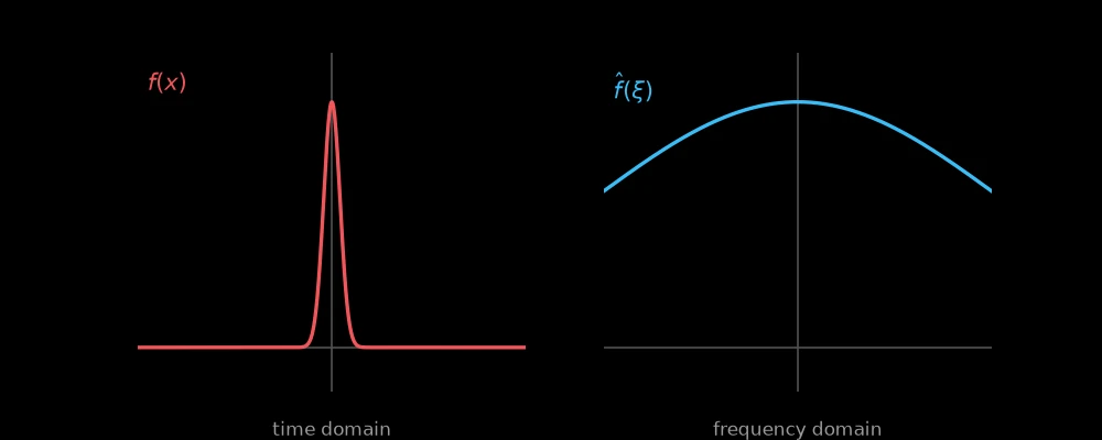
Concentrated in time (left) means spread out in frequency (right).

Now consider a sustained, pure tone with a single frequency $\nu$. We end up with a function that might locally look something like $f(x) = \sin(\nu x)$; but this is just a single coefficient in Fourier space, so the frequency spectrum $\hat f(\xi)$ sharpens into a tight spike right around $\xi = \nu$ (and a mirror image at $-\nu$, since Euler’s formula tells us a real tone is a sum of two complex exponentials).

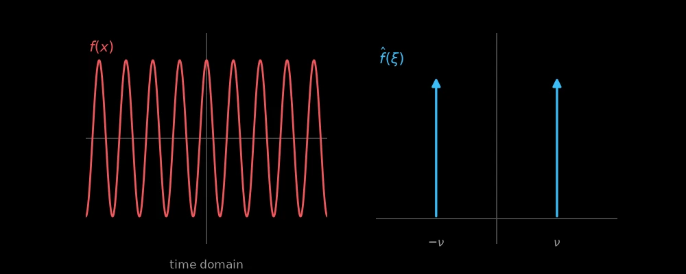
Sustained in time (left) means concentrated in frequency (right).

A tone that’s genuinely eternal would need to concentrate infinitely, which is why it doesn’t satisfy absolute integrability and the integral fails to converge. (This can be remedied with the theory of distributions, which is too much for me to cover here.)

Worked Example: The Rectangular Pulse

The definition is easier to trust once you’ve watched it run. Take a rectangular pulse of duration $T$, equal to $1$ for $\lvert x \rvert \le T/2$ and $0$ otherwise. Its transform is a direct integral:

\[\hat f(\xi) = \int_{-T/2}^{T/2} e^{-2\pi i \xi x}\, dx = \left[\frac{e^{-2\pi i \xi x}}{-2\pi i \xi}\right]_{-T/2}^{T/2} = \frac{e^{\pi i \xi T} - e^{-\pi i \xi T}}{2\pi i \xi} = \frac{\sin(\pi \xi T)}{\pi \xi}\]

This is $T \operatorname{sinc}(\xi T)$, where $\operatorname{sinc}(u) = \sin(\pi u)/(\pi u)$: a central spike of height $T$ at $\xi = 0$ whose first zeros sit at $\xi = \pm 1/T$. A pulse lasting twice as long has a spike half as wide. That’s the time-frequency tradeoff in one formula: duration times bandwidth is a constant.

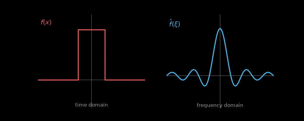
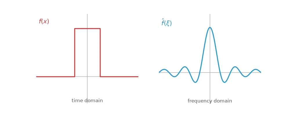A rectangular pulse (left) and its sinc-shaped transform (right).

The finite-duration tone from the main text is the same computation with a twist. Multiplying $f$ by $e^{2\pi i \nu x}$ shifts its transform, since

\[\int_{-\infty}^{\infty} f(x)\, e^{2\pi i \nu x}\, e^{-2\pi i \xi x}\, dx = \hat f(\xi - \nu)\]

so a pure oscillation at frequency $\nu$ that lasts for time $T$ has transform $T \operatorname{sinc}((\xi - \nu) T)$: the same spike, moved to $\xi = \nu$, and narrowing as $T$ grows. A real tone $\cos(2\pi \nu x)$ is half of $e^{2\pi i \nu x}$ plus half of $e^{-2\pi i \nu x}$, so it produces two spikes, at $\pm\nu$.

You may be sensing a theme: “sharpness” in one domain causes “blur” in the other. This isn’t a limitation of the Fourier transform, it’s a fact about the signal itself.

This is the general idea behind the uncertainty principle, which is most famously expressed in physics as a relationship between the position and momentum of an electron. These functions are Fourier conjugates: one is the Fourier transform of the other.

Because these are measurements, we only ever have a probability distribution for position and a probability distribution for momentum; both of these are typically Gaussians. But if one Gaussian has very low variance, meaning that we have a high degree of certainty about its value, then the other must have proportionately high variance, meaning we’re very uncertain about its true value. The proof of this is a straightforward calculation, and it also implies that the Fourier transform of a Gaussian is another Gaussian. (In other words, it’s a fixed point of the Fourier transform.)

Worked Example: The Gaussian

The Gaussian $f(x) = e^{-\pi x^2}$ is the second classic example of a Fourier transform, because $\hat f(\xi) = e^{-\pi \xi^2}$. (Completing the square in the exponent, $-\pi x^2 - 2\pi i \xi x = -\pi(x + i\xi)^2 - \pi \xi^2$, pulls out the factor $e^{-\pi \xi^2}$, and the remaining integral is the usual $\int e^{-\pi u^2}\, du = 1$ after a contour shift.) Rescaling shows the same tradeoff: $e^{-\pi a x^2}$ transforms to $a^{-1/2} e^{-\pi \xi^2 / a}$, so a wide Gaussian in time is a narrow one in frequency and vice versa.

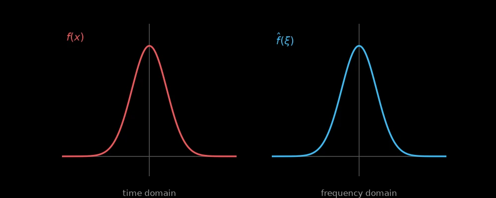
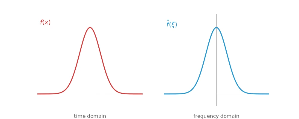The Gaussian is its own Fourier transform.

Written as $e^{-x^2/(2\sigma^2)}$, the standard form of a Gaussian bump with variance $\sigma^2$, $f(x) = e^{-\pi a x^2}$ has $\sigma_x^2 = \frac{1}{2\pi a}$, and its transform $\hat f(\xi) = a^{-1/2} e^{-\pi \xi^2 / a}$ has $\sigma_\xi^2 = \frac{a}{2\pi}$. Multiply the two together and $a$ cancels completely:

\[\sigma_x^2\, \sigma_\xi^2 = \frac{1}{2\pi a} \cdot \frac{a}{2\pi} = \frac{1}{4\pi^2}\]

This is a fixed constant no matter how $f$ or $\hat f$ are rescaled: the variances are exactly inversely proportional, $\sigma_\xi^2 = \dfrac{1}{4\pi^2 \sigma_x^2}$, shrink one and the other grows to compensate. The Gaussian is the extreme case, the exact analogue of a minimum-uncertainty state in quantum mechanics: no function packs a smaller product of time and frequency spread.

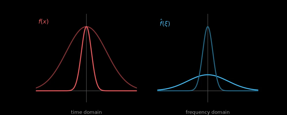
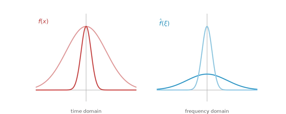Whichever Gaussian is narrow in time is wider in frequency and vice versa.

Conclusion

The Fourier transform is often roughly described as a change of basis, presumably with the pure oscillations as the basis:

\[\ldots, e^{-4\pi i x/p}, \; e^{-2\pi i x/p}, \; 1, \; e^{2\pi i x/p}, \; e^{4\pi i x/p}, \ldots = \left\lbrace e^{2\pi i n x/p} \right\rbrace_{n \in \Z}\]

This isn’t entirely correct, but it captures a fundamental idea. I answer the full question, as well as introduce some higher-level linear algebra, in Is the Fourier Transform a Change of Basis?

But if you don’t care so much about theoretical minutiae, not only do I not blame you, I have another article you might be interested in instead if you’re more applications-minded. The Fast Fourier Transform (FFT for short) is one of a handful of algorithms that underpins the modern world, and is how Fourier’s work actually connects to applications like radar, sonar, radio, and audio that I described earlier. If you’re interested in that, please check out What is the Fast Fourier Transform?