Baby's Second Linear Regression

“Prediction is very difficult, especially if it’s about the future.”
— Niels Bohr

This is the second in a series of articles on linear regression; you can read the first here. This article assumes slightly more familiarity with linear algebra, specifically matrix invertibility and vector spaces. Detailed asides include further prerequisites.

There are several problems that we might encounter in linear regression that damage our model accuracy. Fortunately, many of these problems can not only be solved, but solved in a way that reveals deeper patterns and insights into mathematics and data science.

Polynomial Regression

The first problem is both extremely obvious and very common: perhaps our data just isn’t linear!

The assumption that the underlying function $\textcolor{#38bdf8}{f}$ is linear is quite restrictive; there are many circumstances where we can intuit a nonlinear relationship between the input and output variables. Fortunately, there’s an easy way to extend what we’ve learned about linear regression to cases where we assume $\textcolor{#38bdf8}{f}$ is nonlinear, and can be approximated reasonably well by a polynomial:

\[h(\textcolor{#4ade80}{x}) = \textcolor{#38bdf8}{\theta_0} + \textcolor{#38bdf8}{\theta_1} \textcolor{#4ade80}{x} + \textcolor{#38bdf8}{\theta_2} \textcolor{#4ade80}{x^2} + \cdots + \textcolor{#38bdf8}{\theta_k} \textcolor{#4ade80}{x^k}\]

Crucially, even though our $h$ is non-linear in $\textcolor{#4ade80}{x}$, it’s linear as far as our fitting algorithm is concerned: linearity for fitting purposes is about the relationship between $h$ and its parameters $\textcolor{#38bdf8}{\theta_0}, \textcolor{#38bdf8}{\theta_1}, \ldots, \textcolor{#38bdf8}{\theta_k}$, not between $h$ and $\textcolor{#4ade80}{x}$. We simply define new features by taking powers of our observed data in the $\textcolor{#4ade80}{x}$ column to create new features $\textcolor{#4ade80}{a_1} = \textcolor{#4ade80}{x}$, $\textcolor{#4ade80}{a_2} = \textcolor{#4ade80}{x^2}$, all the way up to $\textcolor{#4ade80}{a_k} = \textcolor{#4ade80}{x^k}$ if we decide we want a degree $k$ polynomial. The same expression is linear with respect to one and nonlinear with respect to the other:

\[h(\textcolor{#4ade80}{x}) = \underbrace{\textcolor{#38bdf8}{\theta_0} + \textcolor{#38bdf8}{\theta_1} \textcolor{#4ade80}{a_1} + \cdots + \textcolor{#38bdf8}{\theta_k} \textcolor{#4ade80}{a_k}}_{\text{linear w.r.t. each } \textcolor{#4ade80}{a_i}} = \underbrace{\textcolor{#38bdf8}{\theta_0} + \textcolor{#38bdf8}{\theta_1} \textcolor{#4ade80}{x} + \cdots + \textcolor{#38bdf8}{\theta_k} \textcolor{#4ade80}{x^k}}_{\text{nonlinear w.r.t. } \textcolor{#4ade80}{x}}\]

That means everything from the first article — the design matrix, the closed form solution $\textcolor{#38bdf8}{\vec \theta} = (\textcolor{#4ade80}{X}^T\textcolor{#4ade80}{X})^{-1}\textcolor{#4ade80}{X}^T\textcolor{#fb7185}{\vec y}$ — carries over unchanged, once $\textcolor{#4ade80}{X}$’s columns are powers of $\textcolor{#4ade80}{x}$ (or cross terms of $\textcolor{#4ade80}{\vec x}$) instead of just $\textcolor{#4ade80}{\vec x}$ itself. This idea of defining new features to capture important relationships (here, nonlinearity) is very powerful, and is called feature engineering.

Multivariable Linear Regression and Omitted Variable Bias

The same idea we’ve used here for single-variable polynomials generalizes very smoothly to multivariable polynomials, so long as we remember to include all the necessary terms. If we have $d$ input variables, we shouldn’t just include powers of each variable on its own (like $\textcolor{#4ade80}{x_1^2}$, $\textcolor{#4ade80}{x_1^3}$, $\textcolor{#4ade80}{x_2^2}$, etc.) because we might miss relationships between the variables, like what the degree $3$ term $\textcolor{#4ade80}{x_1^2x_2}$ might capture. For example, if $\textcolor{#38bdf8}{f}$ depends heavily on $\textcolor{#4ade80}{x_1^2x_2}$, but our $h$ only has $\textcolor{#4ade80}{x_1^2}$, $\textcolor{#4ade80}{x_1^3}$, and $\textcolor{#4ade80}{x_2}$, then not only are we underfitting because we fail to capture a specific relationship between $\textcolor{#4ade80}{x_1}$ and $\textcolor{#4ade80}{x_2}$, but the coefficients that we do try to fit for those single-variable terms will try (and almost always fail) to account for that missing $\textcolor{#4ade80}{x_1^2x_2}$ term. This biases those coefficients, skewing their ability to represent the single-variable relationships that they’re supposed to account for, and our overall model will be much less accurate.

The weird distortion caused by forgetting to include the cross-terms is called omitted-variable bias. All this is to say, if we want to fit a degree $k$ polynomial regression, we must include all cross terms of degree $k$ or below. This means we often add in many new terms; if we suspect some of those terms are extraneous, there’s a better solution than omitting them (which we’ll discuss in the section on ridge regression).

Problems

Multicollinearity

A major problem we’re likely to encounter in polynomial regression is that all of our new polynomial features are highly correlated with each other: obviously there’s going to be a relationship between features like $\textcolor{#4ade80}{x_1^2}$ and $\textcolor{#4ade80}{x_1^3}$, because they’re both determined by $\textcolor{#4ade80}{x_1}$! This is also true of our other features like $\textcolor{#4ade80}{x_1x_2}$ and $\textcolor{#4ade80}{x_1^2x_2}$. The situation where we have many variables that are highly dependent is called (multi)collinearity.

Returning to the closed form solution to standard linear regression from the last article — since we’re going to be experimenting with alternatives to ordinary least squares later in this article, we’ll call this solution the normal equation:

\[\textcolor{#38bdf8}{\vec\theta} = (\textcolor{#4ade80}{X}^T\textcolor{#4ade80}{X})^{-1}\textcolor{#4ade80}{X}^T\textcolor{#fb7185}{\vec y}\]

you might notice that the normal equation requires $\textcolor{#4ade80}{X}^T\textcolor{#4ade80}{X}$ to be invertible. Non-invertibility, called singularity, means that some of the equations represented by our data are redundant; perfectly collinear columns repeat the same information, so a matrix inverse can’t exist because two different candidate vectors for $\textcolor{#38bdf8}{\vec\theta}$ produce the same output, and the inverse that determines which $\textcolor{#38bdf8}{\vec\theta}$ we go with has no way to choose between them. Highly correlated columns can push $\textcolor{#4ade80}{X}^T\textcolor{#4ade80}{X}$ “closer” to being singular. In practice this doesn’t usually blow up outright, it just makes $(\textcolor{#4ade80}{X}^T\textcolor{#4ade80}{X})^{-1}$ wildly sensitive: tiny changes in the training data (a different noise draw, one added or removed point, etc.) can swing the fitted coefficients enormously, even while the model’s overall predictions stay reasonable. That instability, not the predictions themselves, is the real symptom of multicollinearity.

Understanding the Volatility with Eigendecompositions

Under the Gauss–Markov assumptions, the covariance of the fitted coefficients is $\mathrm{Var}(\textcolor{#38bdf8}{\hat\theta} \mid \textcolor{#4ade80}{X}) = \sigma^2(\textcolor{#4ade80}{X}^T\textcolor{#4ade80}{X})^{-1}$. Eigendecompose $\textcolor{#4ade80}{X}^T\textcolor{#4ade80}{X} = Q\Lambda Q^T$, so

\[(\textcolor{#4ade80}{X}^T\textcolor{#4ade80}{X})^{-1} = Q\Lambda^{-1}Q^T\]

where $Q$ is orthogonal with columns given by the orthonormal eigenvectors of $\textcolor{#4ade80}{X}^T\textcolor{#4ade80}{X}$, and $\Lambda$ is the diagonal matrix of eigenvalues of $\textcolor{#4ade80}{X}^T\textcolor{#4ade80}{X}$.

So, this equation is telling us that the variance of $\textcolor{#38bdf8}{\hat\theta}$ splits into orthogonal directions, one per eigenvector of $\textcolor{#4ade80}{X}^T\textcolor{#4ade80}{X}$, each scaled by $1/\lambda_i$. If $\textcolor{#4ade80}{X}^T\textcolor{#4ade80}{X}$ is “close to” singular, that means some eigenvalue $\lambda_i$ is close to zero, so the variance of $\textcolor{#38bdf8}{\hat\theta}$ blows up specifically along that direction. This is why tiny changes in the data cause huge swings in the coefficients of our fit.

Understanding the Volatility with Numerical Methods

Recall that for a matrix $A$, the condition number of $A$ is the ratio of its largest singular value to its smallest singular value:

\[\kappa(A) = \|A\|\,\|A^{-1}\| = \sigma_{\max}(A)/\sigma_{\min}(A)\]

where $\lVert A\rVert$ denotes the spectral (operator) norm of $A$.

You can calculate that the condition number of $\textcolor{#4ade80}{X}^T\textcolor{#4ade80}{X}$ is the square of the condition number of $\textcolor{#4ade80}{X}$, so if $\textcolor{#4ade80}{X}$ has even a slightly large condition number, $\textcolor{#4ade80}{X}^T\textcolor{#4ade80}{X}$’s will be massive. Computing $(\textcolor{#4ade80}{X}^T\textcolor{#4ade80}{X})^{-1}$ directly in floating point can amplify rounding error badly enough that the computed $\textcolor{#38bdf8}{\hat\theta}$ doesn’t even accurately solve the normal equation it’s supposed to. In practice, this is often why we sidestep the normal equation using numerical methods rather than literally forming and inverting $\textcolor{#4ade80}{X}^T\textcolor{#4ade80}{X}$.

This volatility is worth taking seriously for at least three reasons, each of which deserves its own section.

Interpretability

The first problem is that it makes the actual model outputs hard to interpret. Typically, linear regression is very nice because we can get clear and very granular information from each of the elements in $\textcolor{#38bdf8}{\vec \theta}$ quantifying how large the effect each $\textcolor{#4ade80}{x}$ variable has on $\textcolor{#fb7185}{y}$. This is why some industries, like quantitative finance, have started preferring linear models over neural networks (which are famously almost impossible to interpret).

However, if our volatility is high, then $\textcolor{#38bdf8}{\vec \theta}$ can vary wildly based on training data — even the sign can flip! — and it’s hard to say anything about $\textcolor{#38bdf8}{f}$ when our $\textcolor{#38bdf8}{\vec \theta}$ is so sensitive to the noise $\epsilon$.

The Bias-Variance Tradeoff

The second reason we dislike high volatility is that a large variance in $\textcolor{#38bdf8}{\theta}$ may cause our model to generalize poorly even when our (mean-square) error is low on the training data; in other words, our coefficients are too sensitive to the specific sample they were fit on. You may recognize this as overfitting, which we introduced in the first article.

You can experiment a bit with an overfitting model here: notice how dragging the degree slider up gives the model enough freedom to fit every point, and training error converges to 0. Because we generated this data ourselves, we can see from the graph that the true $\textcolor{#38bdf8}{f}$ needs a polynomial around degree 4 or 5 for the best fit, but you may notice that even at the “optimal” degrees our out-of-sample accuracy can fluctuate wildly when we generate many different data sets; we still seem to be overfitting even when we know the right value of $k$. If we didn’t know the true value of $k$ (which we rarely do in practice), we’d be hosed; this is the danger of high volatility.

Degree: 3

Train MSE: · Test MSE:

There’s a deeper relation at play here between degree of the polynomial and the high variance we’re seeing, and which generalizes to almost any machine learning model you’re likely to encounter: the bias-variance tradeoff.

\[\underbrace{\mathbb{E}\big[(\textcolor{#fb7185}{y_0} - \hat h(\textcolor{#4ade80}{x_0}))^2\big]}_{\text{expected test MSE}} = \underbrace{\big(\textcolor{#38bdf8}{f}(\textcolor{#4ade80}{x_0}) - \bar h(\textcolor{#4ade80}{x_0})\big)^2}_{\text{Bias}[\hat h(x_0)]^2} + \underbrace{\mathrm{Var}[\hat h(\textcolor{#4ade80}{x_0})]}_{\text{sensitivity to the sample}} + \underbrace{\sigma^2}_{\text{irreducible noise}}\]

This equation tells us that the amount of error we expect from our model (left hand side) is equal to the bias of our model plus the variance of our model, plus some extra error represented by how bad our noise $\epsilon$ is (larger variance $\sigma^2$ means more noise).

Deriving the Bias-Variance Decomposition

Fix a test point $\textcolor{#4ade80}{x_0}$ with true response $\textcolor{#fb7185}{y_0} = \textcolor{#38bdf8}{f}(\textcolor{#4ade80}{x_0}) + \epsilon$, where $\epsilon$ is mean-zero noise with variance $\sigma^2$, independent of the training data. Our fitted model’s prediction $\hat h(\textcolor{#4ade80}{x_0})$ is itself random, since it depends on which particular training sample we happened to draw. Write $\bar h(\textcolor{#4ade80}{x_0}) = \mathbb{E}[\hat h(\textcolor{#4ade80}{x_0})]$ for its average over all possible training samples.

Split the prediction error into three pieces:

\[\textcolor{#fb7185}{y_0} - \hat h(\textcolor{#4ade80}{x_0}) = \underbrace{\big(\textcolor{#38bdf8}{f}(\textcolor{#4ade80}{x_0}) - \bar h(\textcolor{#4ade80}{x_0})\big)}_{A} + \underbrace{\big(\bar h(\textcolor{#4ade80}{x_0}) - \hat h(\textcolor{#4ade80}{x_0})\big)}_{B} + \underbrace{\epsilon}_{C}\]

$A$ is a fixed number: how far the average model is from the truth. $B$ is random through the training sample, with $\mathbb{E}[B] = 0$ by construction. $C$ is random through the test-point noise, with $\mathbb{E}[C] = 0$, and independent of $B$. Squaring and taking expectations,

\[\mathbb{E}\big[(A+B+C)^2\big] = A^2 + \mathbb{E}[B^2] + \mathbb{E}[C^2] + 2A\,\mathbb{E}[B] + 2A\,\mathbb{E}[C] + 2\,\mathbb{E}[B]\mathbb{E}[C]\]

every cross term vanishes, since $\mathbb{E}[B] = \mathbb{E}[C] = 0$ and $B \perp C$. What’s left is

\[\mathbb{E}\big[(\textcolor{#fb7185}{y_0} - \hat h(\textcolor{#4ade80}{x_0}))^2\big] = A^2 + \mathbb{E}[B^2] + \mathbb{E}[C^2] = \big(\textcolor{#38bdf8}{f}(\textcolor{#4ade80}{x_0}) - \bar h(\textcolor{#4ade80}{x_0})\big)^2 + \mathrm{Var}[\hat h(\textcolor{#4ade80}{x_0})] + \sigma^2\]

While we don’t control the irreducible noise (as the name indicates), we do decide the model $h$, like with the degree slider in the demo. $h$, of course, determines how bad the bias and the variance are.

Unfortunately, less bias means more variance, and less variance means more bias. Both bias and variance are bad. However, their relationship is almost always nonlinear, so it’s possible to find a model $h$ such that the bias and variance together are minimized. The chart below tracks exactly this for the demo above: for every polynomial degree, Bias² and Variance are computed for real (many refits on fresh noisy samples from that demo’s own true curve), and the dashed line follows wherever you last left the degree slider.

Full range, log scale

Bias² Variance Total expected error

Clamped to degrees 1–6, linear scale

Bias² Variance Total expected error

You may notice there’s a sweet spot around $k = 4$ or $5$, where bias is decreasing and variance is increasing, but bias + variance is at a global minimum. This is the sweet spot we want to find; we’ll discuss additional settings we can tweak to find this minimum shortly.

Out-of-Sample Inaccuracy

The first two reasons that volatility is bad have both focused on overfitting generally, but the final reason to avoid volatility is that it has higher error on specific kinds of out-of-sample data.

To be a bit more precise, if we have a lot of features, then our model will naturally recognize classes of data where specific features tend to group together. Densely represented classes — where the training data thoroughly covers that region of feature space — generalize well to new out-of-sample points. However, there will inevitably be some classes of data that are only sparsely represented. Standard linear regression is bad at generalizing on these sparse classes, because ordinary least squares makes very unreliable and volatile estimates when it has little data.

(If you read the eigendecomposition aside above, “classes of data” refers to data that tends to be collinear with the eigenvectors of $\textcolor{#4ade80}{X}^T\textcolor{#4ade80}{X}$ that have the smallest associated eigenvalues. Smaller eigenvalues cause larger volatility, so these collinear sample vectors are the most vulnerable to noise.)

Solution: Alternative Regressions

So, our only “solution” thus far is to reduce the complexity of the model, like reducing the degree of our polynomial model. However, this introduces two new major issues:

1. A lower degree hurts our model’s ability to accurately fit the underlying relationship between $\textcolor{#4ade80}{X}$ and $\textcolor{#fb7185}{y}$, limiting our accuracy if the true relationship genuinely needs the extra flexibility.
2. This doesn’t help at all if we’re experiencing high amounts of collinearity in a model that is already linear; although collinearity most often emerges in the context of polynomial models, it can cause issues even when we already want a strictly linear model.

What do we do?

Ridge Regression

One real solution is to change the way that we judge model error, “penalizing” the model for choosing coefficients that are more likely to overfit, without having to change the model’s degree at all. This solution is much more appealing because it doesn’t put a cap on our accuracy the way lowering the degree does, and also doesn’t force us away from a model we think accurately represents the underlying function $\textcolor{#38bdf8}{f}$.

We can apply this “penalty” by modifying our ordinary least squares formula by adding a new term determined by the variable $\textcolor{#94a3b8}{\lambda}$:

\[J(\textcolor{#38bdf8}{\vec\theta}) = \|\textcolor{#4ade80}{X}\textcolor{#38bdf8}{\vec\theta} - \textcolor{#fb7185}{\vec y}\|^2 + \textcolor{#94a3b8}{\lambda} \sum_{i=1}^{k} \textcolor{#38bdf8}{\theta_i}^2\]

$\textcolor{#94a3b8}{\lambda}$ is called a hyperparameter because we decide its value before we start training our model. The sum runs over every coefficient except the $\textcolor{#fb7185}{y}$-intercept $\textcolor{#38bdf8}{\theta_0}$. The intercept is constant and therefore can’t overfit, so we leave it alone. Notice also that $\textcolor{#94a3b8}{\lambda} = 0$ corresponds exactly to ordinary least squares.

(If you’ve seen Lagrange multipliers in a multivariable calculus class, this formula should look familiar; I have an aside in the Norms section below illuminating the connection.)

Deciding on the optimal value for a hyperparameter is just as much an art as a science; with something like linear regression, it’s common to iterate over a range of hyperparameters, train each on the same training data, and compare their accuracies on test data. You may notice this is exactly what we’ve been doing with the polynomial degree $k$, because it’s also a hyperparameter!

$J(\textcolor{#38bdf8}{\vec\theta})$ is still just a sum of squared linear terms, one extra squared term included, so the same normal-equations approach from the last article still works, with one addition: minimizing $J$ gives

\[\textcolor{#38bdf8}{\vec\theta} = (\textcolor{#4ade80}{X}^T\textcolor{#4ade80}{X} + \textcolor{#94a3b8}{\lambda} I)^{-1}\textcolor{#4ade80}{X}^T\textcolor{#fb7185}{\vec y}\]

where $I$ is the identity matrix (with a 0 in the corner corresponding to the un-penalized intercept $\textcolor{#38bdf8}{\theta_0}$). This is exactly the fix for the multicollinearity instability from the last section: adding $\textcolor{#94a3b8}{\lambda} I$ before inverting pushes $\textcolor{#4ade80}{X}^T\textcolor{#4ade80}{X} + \textcolor{#94a3b8}{\lambda} I$ away from singularity, so the matrix stays comfortably invertible and the fitted coefficients stabilize, even when $\textcolor{#4ade80}{X}^T\textcolor{#4ade80}{X}$ alone is nearly singular.

Degree: 3 Ridge λ: 0.00

Train MSE: · Test MSE:

The demo above offers two hyperparameter sliders: one for $\textcolor{#94a3b8}{\lambda}$ and one for the polynomial degree. The real $\textcolor{#38bdf8}{f}$ is complex enough that lowering the degree of our hypothesized model $h$ runs a real risk of underfitting, but collinearity is bad enough that the model is unstable. Increasing $\textcolor{#94a3b8}{\lambda}$ from 0 will stabilize the wild swings, and test error should improve even though the degree hasn’t changed at all: the penalty provides the same benefits as reducing the degree, but it does it by shrinking coefficients toward zero rather than removing terms outright, so we don’t lose flexibility the true curve actually needs.

But if we push $\textcolor{#94a3b8}{\lambda}$ too far, the curve flattens out and stops tracking the true shape at all. Increasing the penalty is our way of telling the model it’s overfitting, so telling it that it’s overfitting too much makes it underfit.

Lasso Regression

There are also cases where we expect most of the parameters $\textcolor{#38bdf8}{\theta_i}$ in our linear regression model to be zero; this is often the case with polynomial regression, which forces us to add an enormous number of polynomial terms which are often irrelevant. In general cases, we might also want to focus on a very small number of the most predictive features, and be alright with several of the less predictive features being “dropped” even if it means a slight penalty to accuracy. This makes for models that require less data, fit in lower-dimensional space, and that humans can very easily interpret and reason about.

Lasso regression (“least absolute shrinkage and selection operator”) takes the same penalty idea as ridge regression, but penalizes the absolute value of $\textcolor{#38bdf8}{\vec\theta}$ instead of its square:

\[J(\textcolor{#38bdf8}{\vec\theta}) = \|\textcolor{#4ade80}{X}\textcolor{#38bdf8}{\vec\theta} - \textcolor{#fb7185}{\vec y}\|^2 + \textcolor{#94a3b8}{\lambda} \sum_{i=1}^{k} \lvert\textcolor{#38bdf8}{\theta_i}\rvert\]

with the size of the penalty again being controlled by the hyperparameter $\textcolor{#94a3b8}{\lambda}$.

We can see how, like ridge, this regression strategy forces the coefficients $\textcolor{#38bdf8}{\theta_i}$ towards zero: smaller coefficients clearly makes for a smaller penalty. What isn’t clear is why this forces many coefficients to be exactly zero when $\textcolor{#94a3b8}{\lambda}$ is large.

The answer recalls the graphs of $y = \lvert x\rvert$ versus $y = x^2$; they both decrease, have a global minimum at $x = 0$, then increase. But $\lvert x \rvert$ has a corner at $x = 0$, whereas $x^2$ is smooth; this difference in geometry is the key.

The unconstrained minimum is the $\textcolor{#38bdf8}{\vec \theta_{\text{OLS}}}$ that ordinary least squares would have us choose. Remembering that vectors have a nice spatial intuition, let’s picture it living in a coordinate space that represents all the possible values of $\textcolor{#38bdf8}{\theta}$ that we could choose for our solution. Let’s call this whole space $\textcolor{#38bdf8}{\vec\theta}$-space, and denote the unconstrained minimum that OLS produces $\textcolor{#38bdf8}{\vec \theta_{\text{OLS}}}$ for the remainder of this section.

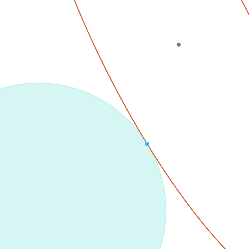
The penalty that ridge regression adds is equivalent to adding an additional constraint: any ridge solution has to have $\sum \textcolor{#38bdf8}{\theta_i^2}\ \leq t$ for some $t$ depending on $\textcolor{#94a3b8}{\lambda}$. Just like how the graph of $y = x^2$ generates a parabola, this algebraic constraint essentially generates an ellipse around the origin that geometrically restrains the ridge solution inside its borders, so the optimal ridge solution is the value of $\textcolor{#38bdf8}{\vec\theta}$ inside the ellipse that is “closest” to the OLS’s optimal $\textcolor{#38bdf8}{\vec\theta_{\text{OLS}}}$. Let’s call this solution $\textcolor{#38bdf8}{\vec \theta_{\text{ridge}}}$.

The ellipse’s tangent point keeps both coefficients nonzero: $\textcolor{#38bdf8}{\vec\theta_{\text{ridge}}}$ shrinks toward the origin but lands off either axis.

Lasso, on the other hand, has a different penalty that corresponds to the constraint $\sum \lvert\textcolor{#38bdf8}{\theta_i}\rvert \leq t$; just like how $y = \lvert x \rvert$ generates a corner, this constraint generates a diamond around the origin that constrains the lasso solution inside its borders. However, the corners of the diamond are exactly aligned with the “directions” of $\textcolor{#38bdf8}{\vec\theta}$-space that force individual components of $\textcolor{#38bdf8}{\vec\theta}$ to be zero. (In other words, these corners are situated on the standard basis vectors of $\textcolor{#38bdf8}{\vec\theta}$-space.) Because an optimal solution is typically going to end up on a corner if $\textcolor{#94a3b8}{\lambda}$ is large enough (equivalent to $t$ being small enough), a large $\textcolor{#94a3b8}{\lambda}$ forces the elements of $\textcolor{#38bdf8}{\vec\theta_{\text{lasso}}}$ to zero.

The diamond’s tangent point lands exactly on a vertex: $\textcolor{#38bdf8}{\vec\theta_{\text{lasso}}}$’s second coefficient isn’t shrunk close to zero, it’s exactly zero.

You can see in the diagrams above that the corners of the diamond poke out farther than the flat sides, so the corners (which always align with some elements of $\textcolor{#38bdf8}{\vec\theta}$ being zero) are almost always closest to the unconstrained minimum $\textcolor{#38bdf8}{\vec\theta_{\text{OLS}}}$; in contrast, the ellipse generated by ridge’s restraints bows out, so it’s relatively unlikely for $\textcolor{#38bdf8}{\vec\theta_{\text{ridge}}}$ to be exactly zero.

What’s with that ellipse around $\textcolor{#38bdf8}{\vec\theta_{\text{OLS}}}$?

Picture $J(\textcolor{#38bdf8}{\vec\theta}) = \lVert\textcolor{#4ade80}{X}\textcolor{#38bdf8}{\vec\theta} - \textcolor{#fb7185}{\vec y}\rVert^2$ itself as a bowl over $\textcolor{#38bdf8}{\vec\theta}$-space, with $\textcolor{#38bdf8}{\vec\theta_{\text{OLS}}}$ sitting at the bottom. A level set (or contour) of that bowl at height $c$ is $\lbrace\textcolor{#38bdf8}{\vec\theta} : J(\textcolor{#38bdf8}{\vec\theta}) = c\rbrace$ — a closed curve around $\textcolor{#38bdf8}{\vec\theta_{\text{OLS}}}$, an ellipse in this two-coefficient picture. Every point on it has exactly the same loss $c$; a curve farther from $\textcolor{#38bdf8}{\vec\theta_{\text{OLS}}}$ means higher loss everywhere on it.

The curve drawn in each figure is a single level set, at the one height $c^\ast$ that the constrained solution actually achieves — not a candidate picked out of several. Finding $\textcolor{#38bdf8}{\vec\theta_{\text{ridge}}}$ or $\textcolor{#38bdf8}{\vec\theta_{\text{lasso}}}$ never involves comparing a family of contours against the region; both come from gradient descent directly on the continuous bowl, projected back into the region at every step, which converges straight to a point. The curve is drawn afterward, purely to show which level set that point happens to land on.

That value $c^\ast$ isn’t arbitrary, though. Any curve at a lower loss than $c^\ast$ never reaches the shaded region at all, so it isn’t achievable subject to the constraint; any curve at a higher loss is settling for more than necessary, since $c^\ast$ is already reachable. $c^\ast$ is the smallest achievable loss, full stop, and the point where its curve first touches the region’s boundary is exactly the constrained solution.

This is also what “closest” to $\textcolor{#38bdf8}{\vec\theta_{\text{OLS}}}$ actually means above: not closest in the ordinary Euclidean, ruler-and-compass sense, but closest in loss — sitting on the lowest-$c$ contour that’s reachable at all. Those two notions of “closest” agree only when the bowl’s contours are perfect circles, i.e. when $\textcolor{#4ade80}{X}^T\textcolor{#4ade80}{X}$ happens to be a multiple of the identity. These figures deliberately use correlated features (the same kind of correlation from the Multicollinearity section), so their contour comes out as a tilted ellipse instead — which is exactly why $\textcolor{#38bdf8}{\vec\theta_{\text{ridge}}}$ isn’t the Euclidean-nearest point in the disk to $\textcolor{#38bdf8}{\vec\theta_{\text{OLS}}}$, it’s the point where that tilted ellipse first touches the disk’s boundary.

This tangency framing is also why the region’s shape decides whether coefficients hit zero. On the ellipse, the contour touches it along a smooth, curved stretch of boundary, off either axis. On the diamond, the corners poke out farther from the origin than the flat edges between them, so the contour is disproportionately likely to make contact right at a corner instead — and a corner is, by construction, a point where all but one coordinate is exactly zero.

Unfortunately, lasso’s sharp corners break the trick that made ridge regression solvable by a closed-form equation: $\textcolor{#38bdf8}{\theta_i}^2$ is smooth everywhere, so setting $\nabla J = 0$ and solving gave us a single closed-form matrix formula. $\lvert\textcolor{#38bdf8}{\theta_i}\rvert$ has a corner at $\textcolor{#38bdf8}{\theta_i} = 0$ where it isn’t differentiable, so there’s no gradient to set to zero there, and no analogous closed form for lasso. Fitting it means reaching for an iterative numerical method instead; coordinate descent is the usual algorithm of choice, but that’s unfortunately out of scope for this article.

Norms

You might have noticed that both ridge and lasso regression didn’t really change the underlying linear regression algorithm, just the formula we used to calculate loss. What we’ve actually done is keep the algorithm the same, and just changed the norm that we use to calculate the distance between $\textcolor{#38bdf8}{\vec \theta}$ and the origin. Discussing the general theory of norms will help us understand OLS, ridge, and lasso better, as well as lay the foundation to explore different models.

A norm is a function from a vector space to the nonnegative real numbers that has certain properties. Formally, given a real or complex vector space $V$, a function $n: V \to \R_{\geq 0}$ is called a norm if it satisfies the following properties:

1. The triangle inequality (also called subadditivity): $n(v_1 + v_2) \leq n(v_1) + n(v_2)$ for all $v_1, v_2 \in V$.
2. Absolute homogeneity: $n(sv) = \lvert s \rvert n(v)$ where $s$ is a scalar, $\lvert s \rvert$ is the absolute value of $s$, and $v \in V$.
3. Positivity (also called positive definiteness): $n(v) = 0$ if and only if $v$ is the zero vector.

The point is that a norm functions very similarly to a metric on a metric space, if you’ve ever heard of that.

In lay terms, the purpose of a norm is that it provides a spatial relationship between all the vectors in a vector space, and defines the operative word “best” when we say “best fit”.

These norms originate from the mathematical field of real analysis, where we consider infinite-dimensional vector spaces of functions with different norms. In the discrete case, we define the $\ell^p$ norm, for $1 \leq p \leq \infty$, of an $n$-dimensional vector $\textcolor{#4ade80}{\vec x}$ to be

\[\lVert \textcolor{#4ade80}{\vec x} \rVert_p = \left(\sum_{i=1}^n |\textcolor{#4ade80}{x_i}|^p\right)^{1/p}\]

If you plug in $p = 2$, you’ll notice this simplifies down to the Euclidean norm. If we only care about comparing the relative distances of different vectors — specifically, when we’re comparing the accuracies of two different linear regression models — we can skip taking $p$-th roots because they won’t change whether one is greater than the other; you’ll recognize our ordinary least squares formula as the result.

The strategy we used in ridge regression of adding a penalty term is called $\ell^p$ regularization. (In this case specifically, it’s called $\ell^2$ regularization.)

Lagrange Multipliers vs $\ell^p$ Regularization

Lagrange multipliers from a multivariable calculus class only handle equality constraints:

\[g(\textcolor{#38bdf8}{\vec\theta}) = c\]

At a critical point, $\nabla f = \mu \nabla g$ for some multiplier $\mu$, because we can’t improve $f$ without leaving the constraint surface.

However, norms are useful because they help us reason about inequalities, so we need to generalize a bit. The Karush-Kuhn-Tucker (KKT) conditions do exactly that: they apply to the case

\(g(\textcolor{#38bdf8}{\vec\theta}) \leq 0\) Formally, for

\[\min_{\textcolor{#38bdf8}{\vec\theta}} \|\textcolor{#4ade80}{X}\textcolor{#38bdf8}{\vec\theta} - \textcolor{#fb7185}{\vec y}\|^2 \quad\text{subject to}\quad g(\textcolor{#38bdf8}{\vec\theta}) := \|\textcolor{#38bdf8}{\vec\theta}\|_2^2 - t \leq 0\]

the KKT conditions are three requirements on the optimum $\textcolor{#38bdf8}{\vec\theta}^*$ and a multiplier $\mu$:

1. (Stationarity) $\nabla f(\textcolor{#38bdf8}{\vec\theta}^*) + \mu \nabla g(\textcolor{#38bdf8}{\vec\theta}^*) = 0$
2. (Dual feasibility) $\mu \geq 0$
3. (Complementary slackness) $\mu \, g(\textcolor{#38bdf8}{\vec\theta}^*) = 0$

Stationarity is the same condition as ordinary Lagrange multipliers; only the latter two are new: we require $\mu$ to be nonnegative, and either $\mu = 0$ (the constraint is slack, not binding) or $g(\textcolor{#38bdf8}{\vec\theta}^*) = 0$ (the constraint is active, sitting exactly on the boundary). We always have one, but never both; we have this slack because if the unconstrained minimum already satisfies the inequality, there’s nothing to enforce.

We can use these conditions to re-derive our formula for ridge regression: plugging in $f(\textcolor{#38bdf8}{\vec\theta}) = \lVert\textcolor{#4ade80}{X}\textcolor{#38bdf8}{\vec\theta} - \textcolor{#fb7185}{\vec y}\rVert^2$ and $g(\textcolor{#38bdf8}{\vec\theta}) = \lVert\textcolor{#38bdf8}{\vec\theta}\rVert_2^2 - t$ and taking gradients, we get $\nabla f = 2\textcolor{#4ade80}{X}^T\textcolor{#4ade80}{X}\textcolor{#38bdf8}{\vec\theta} - 2\textcolor{#4ade80}{X}^T\textcolor{#fb7185}{\vec y}$ and $\nabla g = 2\textcolor{#38bdf8}{\vec\theta}$. Stationarity becomes

\[2\textcolor{#4ade80}{X}^T\textcolor{#4ade80}{X}\textcolor{#38bdf8}{\vec\theta} - 2\textcolor{#4ade80}{X}^T\textcolor{#fb7185}{\vec y} + 2\mu\textcolor{#38bdf8}{\vec\theta} = 0 \quad\Longrightarrow\quad \textcolor{#38bdf8}{\vec\theta} = (\textcolor{#4ade80}{X}^T\textcolor{#4ade80}{X} + \mu I)^{-1}\textcolor{#4ade80}{X}^T\textcolor{#fb7185}{\vec y}\]

which is exactly the ridge solution with $\mu$ playing the role of $\textcolor{#94a3b8}{\lambda}$. So $\textcolor{#94a3b8}{\lambda}$ isn’t just analogous to a Lagrange multiplier, solving the penalized problem for a given $\textcolor{#94a3b8}{\lambda}$ and solving the constrained problem for whatever $t$ makes $\mu = \textcolor{#94a3b8}{\lambda}$ produce the identical $\textcolor{#38bdf8}{\vec\theta}$.

Complementary slackness tells us something concrete, too: for any $\textcolor{#94a3b8}{\lambda} > 0$, the ridge solution sits exactly on the boundary $\lVert\textcolor{#38bdf8}{\vec\theta}^*\rVert_2^2 = t$, matching the tangent-point picture from the Lasso section above, just for the $\ell^2$ ball instead of the $\ell^1$ diamond.

Dual feasibility ($\mu \geq 0$) does the heavy lifting here: it guarantees the loss’s gradient always points back into the constraint region at the optimum, which is exactly why turning up $\textcolor{#94a3b8}{\lambda}$ only ever shrinks $\textcolor{#38bdf8}{\vec\theta}$ toward the origin, never pushes it away. An equality-constraint Lagrangian has no such guarantee.

Lasso regression corresponds to using the $\ell^1$ norm. This norm lacks a couple nice properties that the $\ell^2$ norm has, but in cases where we want to perform a lasso regression we typically don’t care.

As a final fun fact about $\ell^p$ norms, you might notice that we allow $p=\infty$. Taking limits, we see that the $\ell^\infty$ norm of a vector is simply the maximum of the absolute values of each of its entries:

\[\lVert \textcolor{#4ade80}{\vec x} \rVert_\infty = \max(|\textcolor{#4ade80}{x_1}|, |\textcolor{#4ade80}{x_2}|, \ldots, |\textcolor{#4ade80}{x_n}|)\]

(Proving this is a standard exercise in a first course in measure theory!)

The $\ell^\infty = \max$ norm is very rarely useful in machine learning; it’s usually only used when we care about just looking at the most extreme behavior in a data set, but you can verify that it does indeed satisfy all the requirements to be a norm, and it’s always neat to connect seemingly unrelated functions.

What functions can (non)linear regression actually fit?

You may have noticed that we expanded our attention from fitting functions $f$ that are continuous and linear (in the first article) to the much vaguer class of functions that can be “well-approximated by a polynomial” (at the start of this article). Having discussed norms, we can provide a precise statement for what kinds of $f$ linear regression can fit.

The short of it is that, given enough high-quality data and an appropriate fitting method, linear regression can well-approximate any function in $L^2[a,b]$: that is, $f : \R \to \R$ has to be square-integrable on $[a, b]$, meaning $\int_a^b f(x)^2 \, dx$ exists and is finite.

This comes from two theorems, one in measure theory and one in real analysis. The first is a corollary of Lusin’s theorem:

Continuous functions are dense in $L^2[a,b]$.

By “dense in $L^2[a,b]$”, we roughly mean “common enough that they can approximate any other square-integrable function arbitrarily well”. We can then extend this further to approximation by polynomials with the Weierstrass approximation theorem:

Let $f: \R \to \R$ be continuous on [a, b]. Then for any $\epsilon > 0$, there exists a polynomial $p$ such that for all $x \in [a, b]$, we have $

f(x) − p(x)

< \epsilon$.

This is an incredibly powerful result, and tells us that so long as $f$ is continuous, then the only strict upper limit on how well we can fit $f$ is the quality of our data set and our fitting methods rather than the form of $f$ itself.

At this point, you should object that both of these theorems require knowing $f$, which we obviously don’t in practice; we only have $n$ noisy samples of $f$, so we should be much more concerned with estimating $f$ based on those samples.

We’ve already proven existence; now, we want to cook up a basic construction. Consider a fitting algorithm where we let the polynomial degree $k$ grow with the sample size $n$: the bias-variance tradeoff tells us that we can reduce the MSE by reducing the bias and variance. From our discussion on density above, we see that increasing $k$ drives the bias to zero. Variance, on the other hand, is determined by how many free parameters we’re fitting per data point, so keeping $k$ small relative to $n$ drives the variance to zero. By growing the degree slowly enough ($k \to \infty$ but $k/n \to 0$) both bias and variance will vanish: the fitted polynomial converges to $f$ in mean-square error for any square-integrable $f$, continuous or not, as $n \to \infty$. Statisticians call this a sieve estimator.

(If you want more, see Newey, “Convergence Rates and Asymptotic Normality for Series Estimators,” Journal of Econometrics 79(1), 1997, for the polynomial-regression version made precise.)

This sieve estimator is actually just our polynomial OLS algorithm where we increase the polynomial degree with the number of samples collected. To conclude, given sufficient data, ordinary least squares will be able to fit any square-integrable $f$.

But we’re doing data science here, not pure math; let’s look at an example where we can apply our knowledge to hand-roll a unique norm based on the data we’re given.

Heteroskedasticity: There’s Variance In My Variance!

Every model we’ve discussed so far has assumed the noise $\epsilon^{(i)}$ has the same spread everywhere: $\sigma$ is constant, no matter what $\textcolor{#4ade80}{\vec x^{(i)}}$ is. This situation is called homoskedasticityFrom Greek homós, "same," and skedánnymi, "to scatter." Coined by statistician Karl Pearson in 1905., and is often an unreasonable assumption. Household spending is a classic example: a household with a small income has little room to deviate from a tight, predictable budget, but a household with a large income might save almost all of it one month and blow through a huge chunk of it the next. The noise around the trend line genuinely gets wider as the input grows. This uneven spread is called heteroskedasticityFrom Greek héteros, "different," plus the same skedánnymi, "to scatter.".

You can often spot it directly in a residual plot: instead of scattering evenly above and below zero across the whole range of $\textcolor{#4ade80}{x}$, the residuals fan out into a cone or funnel shape as $\textcolor{#4ade80}{x}$ grows.

The variance also doesn’t have to just increase or decrease; it can fluctuate like a sine wave, polynomial, etc. In this example, it forms a bell curve, with the worst noise in the middle of our $\textcolor{#4ade80}{x}$ values:

Weighted Linear Regression

Heteroskedasticity is exactly the situation weighted least squares was built for. If we have a rough sense of each point’s own noise variance $(\sigma^{(i)})^2$, set $w^{(i)} = 1/(\sigma^{(i)})^2$ so noisier points count for less and cleaner points count for more in the fit. This gives us a weighted norm $\lVert \vec v \rVert_W$, which we can then use to define a weighted residual sum of squares:

\[J(\textcolor{#38bdf8}{\vec \theta}) = \lVert \textcolor{#4ade80}{X}\textcolor{#38bdf8}{\vec\theta} - \textcolor{#fb7185}{\vec y} \rVert_W^2 = \displaystyle{\sum_{i = 1}^n} w^{(i)} (h_{\textcolor{#38bdf8}{\theta}}( \textcolor{#4ade80}{x^{(i)}}) - \textcolor{#fb7185}{y^{(i)}})^2\]

As with earlier loss functions, it would make it easier to study these equations and do our calculations if we could put this norm into a matrix equation just like we did with ordinary least squares and ridge regression. If we define an $n \times n$ diagonal matrix $W$ by

\[W = \text{diag}\left(1/(\sigma^{(1)})^2, \ldots, 1/(\sigma^{(n)})^2\right)\]

then we get a lovely weighted inner product:

\[\langle \vec v, \vec u \rangle _W := \vec u^T W \vec v\]

This is essentially the dot product of two vectors $\vec u$ and $\vec v$ where we weight some of the summands in the dot product more or less than others, according to the corresponding entry in $W$. Setting both arguments to the same vector recovers the weighted norm we started with:

\[\lVert \vec v \rVert_W^2 = \langle \vec v, \vec v \rangle_W = \vec v^T W \vec v\]

By setting $\vec v = (\textcolor{#4ade80}{X}\textcolor{#38bdf8}{\vec\theta} - \textcolor{#fb7185}{\vec y})$, we can get a matrix form for weighted residual sum of squares:

\[J(\textcolor{#38bdf8}{\vec \theta}) = (\textcolor{#4ade80}{X}\textcolor{#38bdf8}{\vec\theta} - \textcolor{#fb7185}{\vec y})^T W (\textcolor{#4ade80}{X}\textcolor{#38bdf8}{\vec\theta} - \textcolor{#fb7185}{\vec y})\]

Then by similar calculations as in the case of the Euclidean norm, the solution $\text{argmin}_{\textcolor{#38bdf8}{\vec \theta}} J(\textcolor{#38bdf8}{\vec \theta})$ is given by solving for the $\textcolor{#38bdf8}{\vec \theta}$ that gives

\[\textcolor{#4ade80}{X}^TW\textcolor{#4ade80}{X}\textcolor{#38bdf8}{\vec \theta} = \textcolor{#4ade80}{X}^T W \textcolor{#fb7185}{\vec y}\]

which has the closed-form solution $\textcolor{#38bdf8}{\vec\theta} = (\textcolor{#4ade80}{X}^TW\textcolor{#4ade80}{X})^{-1}\textcolor{#4ade80}{X}^TW\textcolor{#fb7185}{\vec y}$.

Using a weighted loss function like WRSS allows us to fit heteroskedastic data very neatly; in the example below, noise peaks towards the edges of $\textcolor{#4ade80}{x}$ so points in the middle are more “trustworthy” (that is, they give a better estimate for $\textcolor{#38bdf8}{f}$’s true values) than the points at the extremes that suffer from heavy noise. Ordinary least squares doesn’t account for the variable noise, and fits our data points as if they’re all equally reliable; toggle on the weighted fit below to compare. Points’ fading opacity indicates how much weight each point gets.

Show weighted fit

True line: · OLS fit: · OLS weighted MSE:

One can similarly imagine weighted ridge regression and weighted lasso regression. I leave those derivations to the reader.

Conclusion

We’ve investigated the flexibility and utility that comes with customizing the norms we use in our linear regression models, and this has allowed us to model nonlinear functions and functions with nonconstant variance, as well as fight overfitting in these cases and many others. Altogether, this covers an enormous amount of ground.

There are yet more situations we can encounter that need specific treatments; even though we’ve discussed nonconstant variance, we’ve still largely assumed that our noise is normally distributed with mean 0. Both of these assumptions can be loosened; there’s a veritable zoo of distributions that our noise can sample from: skewed, long-tailed, and mixture distributions all require unique tools to diagnose and resolve. We may also be interested in reasoning further about our regression models, specifically about their robustness, the confidence intervals they provide, and the “degrees of freedom” that our hyperparameters provide. All of these topics will be covered in Baby’s Third Linear Regression.