Cantor's Diagonal Argument

There are many concepts of infinity in mathematics: infinite limits in calculus, the point at infinity in geometry, sets of infinite measure in measure theory, and — the subject of this article — the infinity of set theory. This concept was illuminated by Georg Cantor (1845 – 1918), who is considered the father of the branch of math known as set theory. I tell the story of his life, and the ridicule his work initially met, in a companion piece, Georg Cantor.

By the 1870s, set theory existed in a relatively primitive state. The concept of a set in mathematics appears relatively simple: it is a collection of objects, like numbers or functions and so on, where any particular object is either a member or not a member. For example, the set \(\{1, 2, 3\}\) contains the numbers \(1, 2,\) and \(3\) and nothing else.

Cantor was the first to deeply investigate whether two infinite sets, the set of natural numbers \(\mathbb{N}\) (which consists of the nonnegative whole numbers \(\{0, 1, 2, 3, ...\}\)) and the set of real numbers \(\mathbb{R}\) (consisting of all numbers with a decimal expansion, like \(0, 3, -1, \pi, 3/4\), and so on) both contained the same number of elements. The number of elements that a set contains is called its cardinality, but I’ll also refer to it informally as the “size” of the set. We denote the cardinality of a set \(S\) by \(\lvert S \rvert\).

Cantor’s question seems silly: to figure out how many elements a set has, just count them out one by one. The set \(\{1, 2, 3\}\) has three objects, the set \(\{\sin(x), \cos(x) \}\) has two, and sets like \(\mathbb{N}\) and \(\mathbb{R}\) obviously have infinitely many elements, so that’s it.

But there’s a reason to doubt that simple explanation. One might be suspicious that every element in \(\mathbb{N}\) is also a member of \(\mathbb{R}\), but the converse is not true: numbers like \(-1\), \(\pi\), and \(\frac{3}{4}\) are clearly not in \(\mathbb{N}\). Could these sets still have the same number of objects even though \(\mathbb{N}\) is a subset of \(\mathbb{R}\)?

For a mathematician, there’s an even more compelling motivation: perhaps there is a better definition of the size of a set than just counting out the elements. Obviously, we’d like sets like \(\{1, 2, 3\}\) to still be defined to have three elements, but maybe this definition could be reworked and expanded to assign meaningful — and different — sizes to infinite sets.

Cantor’s work produced a remarkably clever proof whose central idea has been generalized to other groundbreaking work across mathematics and computer science. This article presents that proof in detail and briefly notes some of its other applications.

The Cardinality of a Set

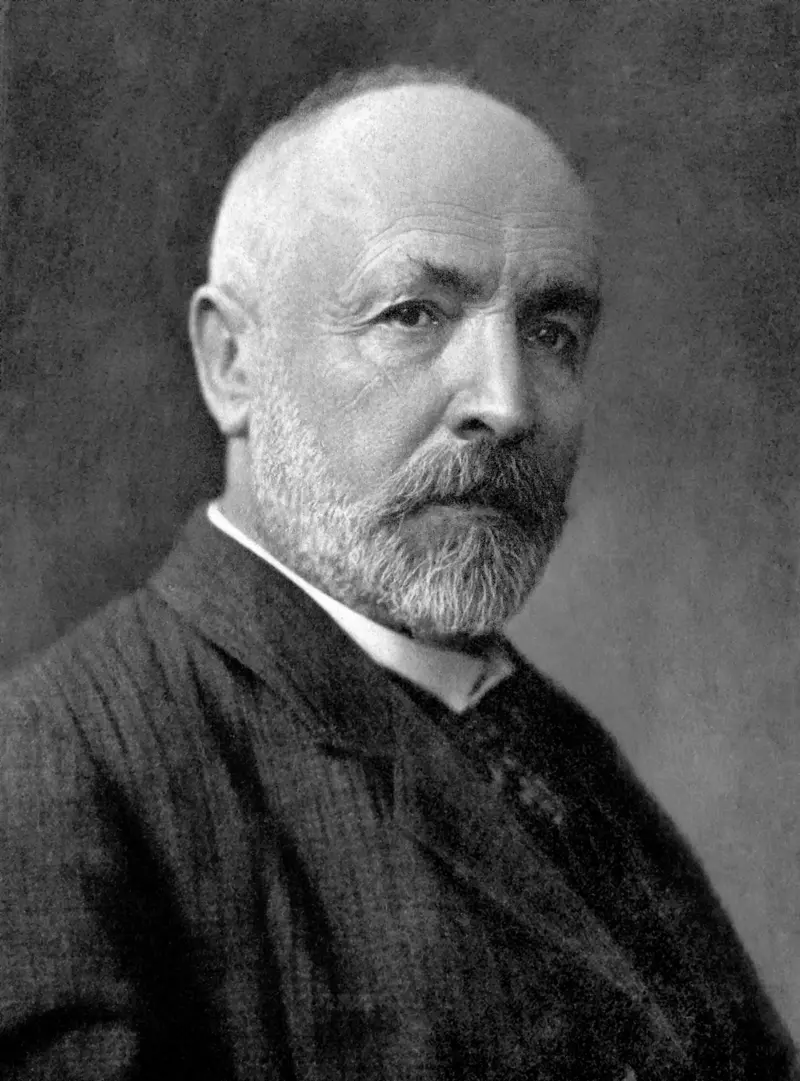Georg Cantor, the father of modern set theory. Public domain, via Wikimedia Commons

The definition of a size of a set that Cantor settled on is actually very intuitive. Imagine that you have a lot of duplicates of the same pair of shoes, but you think you may have lost a couple individual shoes. You might not care about the absolute number of shoes you have remaining, but you do care about whether you have the same number of left and right shoes. In other words, you want to know if the set of left shoes \(L\) is the same size as the set of right shoes \(R\). Besides counting directly, what’s the obvious way to see if one collection is larger than the other?

Pair them up! Every left shoe is the same as every other (their designs are identical, after all) and likewise with every right shoe: we only care if they can all be paired. If we can pair them all up without any shoes being left without a partner, then the sets \(L\) and \(R\) are the same size. If there’s at least one extra left shoe, then \(L\) is larger, and if there’s at least one extra right shoe, then \(R\) is larger.

In the language of mathematics, Cantor wanted to construct a one-to-one correspondence, or a bijection, between the sets \(\mathbb{N}\) and \(\mathbb{R}\).

Definition (Bijection)

A bijection is a function that pairs every element in the domain (the set of all inputs) with exactly one unique element in the codomain (the set of all outputs). Every input must be assigned to exactly one output, no two inputs can have the same output, and every output must be paired with some input. In general, we denote a function \(f\) with domain \(A\) and codomain \(B\) by \(f: A \to B\).

This definition is elegant for two reasons. First, it behaves nicely with finite sets: every set with three elements is in bijection with a set like \(\{1, 2, 3\}\), so we can define some specific formula for a set with \(n\) elements (like \(\{1, 2, ..., n\}\)) and see that if a set has \(n\) elements, it has a bijection with that set.

Second, it allows us to provide a meaningful way in which two infinite sets might (or might not) have the same size, even if they’re both infinite. To start, we can observe that Cantor’s method provides some interesting results.

Example (The Even Natural Numbers)

For example, the set of natural numbers \(\mathbb{N} = \{0, 1, 2, 3, ...\}\) and the set of even natural numbers \(\{0, 2, 4, 6, ...\}\) have the same number of elements, because we can pair them up:

\[\begin{array}{} f(0)&=&0\\ f(1)&=&2\\ f(2)&=&4\\ f(3)&=&6\\ \vdots && \vdots \end{array}\]

This actually makes sense: we can simply take every number in \(\mathbb{N}\) and double it. Clearly the resulting set is \(\{0, 2, 4, 6, ...\}\), and we didn’t add or remove any elements in the process.

Example (The Primes)

Similarly, the set \(\mathbb{N}\) and the set of all prime numbers are the same size:

\[\begin{array}{} f(0)&=&2\\ f(1)&=&3\\ f(2)&=&5\\ f(3)&=&7\\ \vdots && \vdots \end{array}\]

There isn’t an obvious algebraic rule for this set, but the reason is also clear: we can reasonably talk about the first, second, third, and fourth prime, and so on. An elegant proof by Euclid shows that there are infinitely many primes, so intuitively the number of natural numbers and the number of primes is the same.

The idea here is that a set \(S\) is the same size as \(\mathbb{N}\) if we can count out the elements of \(S\) one by one, and every element is eventually counted. If we list the primes in order, then every prime will eventually be enumerated if we keep counting for long enough.

Example (The Integers)

The same is even true for the set of integers \(\mathbb{Z}\) (from the German “Zahlen”, meaning “numbers”), which consists of all whole numbers, including negative numbers: \(\mathbb{Z} = \{..., -2, -1, 0, 1, 2, ...\}\).

There is a simple function that pairs both sets:

\[\begin{array}{} f(0)&=&\hphantom{-}0\\ f(1)&=&\hphantom{-}1\\ f(2)&=&-1\\ f(3)&=&\hphantom{-}2\\ f(4)&=&-2\\ \vdots && \hphantom{-}\vdots \end{array}\]

The function \(f\) can be written out simply:

\[f(n) = \begin{cases} -\dfrac{n}{2} &\text{if } n \text{ is even}\vphantom{\Bigg(} \\ \dfrac{n + 1}{2} &\text{if } n \text{ is odd} \end{cases}\]

Plugging in the different values for \(n\) results in the above table, which obviously lists all the positive and negative integers (and zero). If you’re not convinced that any particular integer \(x\) gets paired with an integer \(n\), then simply plug in \(x = -n/2\) and solve for \(n\) if \(x\) is negative, and plug in \(x = (n+1)/2\) and solve for \(n\) if \(x\) is positive. (This is one instance of a general rule: bijections can be “inverted”: if we have a bijection \(f: A \to B\), we can “invert” it to yield a function \(f^{-1}: B \to A\) such that \(f^{-1}(f(a)) = a\) for all \(a\) in \(A\), and \(f(f^{-1}(b)) = b\). This is why I like the term bijection so much: bijections are bi-directional.)

One final detail: the property of “being the same size” is transitive: if sets \(A\) and \(B\) are the same size, and \(B\) and \(C\) are the same size, then obviously \(A\) and \(C\) are the same size. If we have a bijection \(f: A \to B\) and a bijection \(g: B \to C\), then the function \(g \circ f : A \to C\) (defined by \((g \circ f)(a) = g(f(a))\)) is a bijection between \(A\) and \(C\).

Cantor’s Diagonal Argument

Cantor, now with a logical tool to compare the sizes of infinite sets, would reach one of two outcomes:

1. Constructing (or at least proving the existence of) a correspondence between \(\mathbb{N}\) and \(\mathbb{R}\), or
2. Proving that no correspondence between \(\mathbb{N}\) and \(\mathbb{R}\) could possibly exist.

He ultimately reached the second conclusion with a marvelous new technique of his own creation: Cantor's diagonal argument.

Theorem

There is no bijection between \(\mathbb{N}\) and \(\mathbb{R}\).

This is, in my opinion, one of the most elegant proofs in all of mathematics. The version that I’ll present has three steps:

1. Proving that there is no correspondence between \(\mathbb{N}\) and the interval \((0, 1)\)
2. Proving that there is a correspondence between \((0, 1)\) and \(\mathbb{R}\)
3. Proving that (1) and (2) together show that there is no correspondence between \(\mathbb{N}\) and \(\mathbb{R}\).

There are only two important background details. The first is just clarification: the interval \((0, 1)\) is the set of all real numbers \(r\) strictly between \(0\) and \(1\). Numbers like \(0.0001\), \(0.00012345\), and \(0.7777...\) are all included in \((0, 1)\), but \(0\), \(1\), \(-5\), \(\pi\), and so on are not.

The second (slightly trickier) detail is that (almost) every real number can be expressed uniquely with an infinite decimal expansion. A number like \(0.5\) can be expressed with an infinite number of trailing zeroes, so \(0.5000...\). The only exceptions are numbers that have an infinite number of trailing \(9\)’s: \(0.5999...\) is actually equal to \(0.6\), and \(1\) is actually equal to \(0.9999...\) (yes, really!).

Why does \(0.999\ldots\) equal \(1\)?

This fact is often shocking because people assume real numbers have unique decimal expansions, but they don’t. This is similar to how \(1/2 = 2/4\); there are multiple ways of writing the same number, but with decimal expansions they’re uncommon enough that you might not have encountered them.

The intuitive reason that \(0.999\ldots = 1\) is that there are no numbers between them. Look at the following progression:

\[\begin{array}{rcl} 0.1 &=& 1 - 0.9\\ 0.01 &=& 1 - 0.99\\ 0.001 &=& 1 - 0.999\\ 0.0001 &=& 1 - 0.9999\\ \vdots \hphantom{0.1} &=& \hphantom{0.001} \vdots\\ \end{array}\]

Intuitively, if we have an infinite decimal expansion of \(0.9999\ldots\), then the difference will be an infinite chain of zeroes: \(0.0000\ldots\). (One can make this argument rigorous with a bit of calculus.)

That’s obviously just zero, and two numbers are equal if their difference is zero. This is relevant because it follows that \(1 = 0.9999\ldots\) is not included in the interval \((0,1)\) despite its leading zero!

Now that we’ve laid the groundwork, on to the proof!

Step 1

The first goal is to show that no bijection can possibly exist between \(\mathbb{N}\) and \((0, 1)\). Cantor did this by showing that any general function from \(\mathbb{N}\) to \((0, 1)\) cannot possibly be a bijection, because it will always fail to pair at least one real number.

Proof (No bijection between \(\mathbb{N}\) and \((0, 1)\))

Cantor asks us to consider any arbitrary function \(f: \mathbb{N} \to (0, 1)\). All we know about this function is that it must map \(0\) to some real number in \((0, 1)\) with a particular decimal expansion, and it must map \(1\) to another real number in \((0, 1)\), and so on. He wrote out this map like so:

\[\begin{array}{} f(0) &=& 0.d_{11}d_{12}d_{13}d_{14}\dots\\ f(1) &=& 0.d_{21}d_{22}d_{23}d_{24}\dots\\ f(2) &=& 0.d_{31}d_{32}d_{33}d_{34}\dots\\ f(3) &=& 0.d_{41}d_{42}d_{43}d_{44}\dots\\ \vdots& &\vdots \end{array}\]

Here, \(d_{xy}\) is the \(y\)-th digit (\(0, 1, 2, 3, 4, 5, 6, 7, 8,\) or \(9\)) of the \(x\)-th number. Clearly this function pairs every natural number (on the left) with a real number (on the right), but Cantor devised a clever method to show that the converse is false. He found a way to construct a real number that is not paired up with a natural number:

\[\begin{array}{r|ccccc} \text{digit} & 1 & 2 & 3 & 4 & \cdots \\ \hline f(0) = 0. & {\color{var(--palette-rose)}\boxed{d_{11}}} & d_{12} & d_{13} & d_{14} & \cdots \\ f(1) = 0. & d_{21} & {\color{var(--palette-rose)}\boxed{d_{22}}} & d_{23} & d_{24} & \cdots \\ f(2) = 0. & d_{31} & d_{32} & {\color{var(--palette-rose)}\boxed{d_{33}}} & d_{34} & \cdots \\ f(3) = 0. & d_{41} & d_{42} & d_{43} & {\color{var(--palette-rose)}\boxed{d_{44}}} & \cdots \\ \vdots & \vdots & \vdots & \vdots & \vdots & \ddots \\ \hline 0. & {\color{var(--palette-sky)} n_1} & {\color{var(--palette-sky)} n_2} & {\color{var(--palette-sky)} n_3} & {\color{var(--palette-sky)} n_4} & \cdots \end{array}\]

We assign \({\color{var(--palette-sky)} n_1}\) a digit that is not equal to \({\color{var(--palette-rose)} d_{11}}\), and assign \({\color{var(--palette-sky)} n_2}\) a digit not equal to \({\color{var(--palette-rose)} d_{22}}\), and assign \({\color{var(--palette-sky)} n_3}\) a digit that is not equal to \({\color{var(--palette-rose)} d_{33}}\), and so on, proceeding diagonally. So long as we do not construct a number that ends in an infinite string of nines or zeros (which isn’t hard if we just don’t ever choose \(9\) or \(0\)), then we have constructed a real number which is not assigned to a natural number.

Why are we certain that \(0.{\color{var(--palette-sky)} n_1 n_2 n_3 n_4 \dots}\) doesn’t show up anywhere on the right side? It can’t: its first digit differs from \(f(0)\)’s first digit, its second digit differs from \(f(1)\)’s second digit, and so on. We can see that every real number on the right is guaranteed to differ from the counterexample in at least one place! Because we didn’t assume anything about \(f\) besides that it was a function from \(\mathbb{N}\) to \((0, 1)\), we’ve shown that any function \(f: \mathbb{N} \to (0, 1)\) will always fail to pair at least one real number.

So the sets \(\mathbb{N}\) and \((0,1)\), despite both clearly having an infinite number of elements, do not have the same infinite number of elements.

Step 2

Proof (Bijection between \((0, 1)\) and \(\mathbb{R}\))

Now, we must show that there is a bijection between \((0, 1)\) and \(\mathbb{R}\). We can simply graph one:

\[f(x) = \ln\left(\dfrac{1}{x} - 1\right)\]

Graph of a bijection between \((0, 1)\) and \(\mathbb{R}\)

This function maps every real number between \(0\) and \(1\) to a real number, and a tiny bit of calculus shows that the range of this function spans the entire real line. Equivalently, this function stretches infinitely “up” and infinitely “down” and forms a continuous curve, so it can’t miss any real numbers: any horizontal line will intersect the curve somewhere. Because it’s strictly decreasing, no two inputs are mapped to the same output, and we can conclude \(f\) is a bijection.

There is a nice generalization of step 2, which comes up every so often:

Theorem

For any two real numbers \(a\) and \(b\) with \(a < b\), there are just as many numbers on the interval \((a, b)\) as there are on the entire real line.

Digression: The Fault in The Fault in Our Stars

In particular, there are just as many numbers between \(0\) and \(1\) as there are between \(0\) and \(2\), despite what John Green may tell you:

“There are infinite numbers between 0 and 1. There’s .1 and .12 and .112 and an infinite collection of others. Of course, there is a bigger infinite set of numbers between 0 and 2, or between 0 and a million. Some infinities are bigger than other infinities.”\ — John Green, The Fault in Our Stars

We can see that \((0, 1)\) and \((0, 2)\) have the same cardinality by just taking each number in \((0, 1)\) and doubling it, just like we did with \(\mathbb{N}\) and the even numbers \(\{0, 2, 4, 6, ...\}\). So John is definitely wrong (or at least being sloppy) here, but it’s worth mentioning the concept he’s confusing cardinality with is called measure, which I’ll certainly write about eventually.

I’ve been sitting on that one for a while.

Step 3

This conclusion is extremely short, and finishes the proof by contradiction. Here, we show that if a proposition were true, then a fact that we know to be true would be contradicted, thus showing the proposition to be false. This is essentially a reductio ad absurdum.

Proof (No bijection between \(\mathbb{N}\) and \(\mathbb{R}\))

Assume that a bijection \(g: \mathbb{N} \to \mathbb{R}\) existed.

The bijection \(f: (0, 1) \to \mathbb{R}\) from step (2) has an inverse \(f^{-1}: \mathbb{R} \to (0, 1)\). Composing \(g\) with this inverse gives a bijection \(h = f^{-1} \circ g: \mathbb{N} \to (0, 1)\), defined by \(h(n) = f^{-1}(g(n))\).

We know that such a bijection \(h\) cannot exist by step (1), so our assumption that \(g\) existed must have been wrong. This completes the proof.

The Size(s) of Infinity

Cantor’s revelatory proof showed that there are different sizes of infinite sets. The infinity of \(\mathbb{N}\), the smallest infinity, is denoted \(\aleph_0\) (“aleph null”). In our discussion on prime numbers earlier, I hinted at the idea that any infinite set that can be enumerated also has size \(\aleph_0\): we can count the number of elements in these sets (by assigning them \(0\), \(1\), \(2\), \(3\), etc.) without leaving any numbers out; this is exactly a bijection with \(\mathbb{N}\). We call these infinite sets countably infinite.

The cardinality of \(\mathbb{R}\) is denoted \(2^{\aleph_0}\), or sometimes \(\mathfrak{c}\) (for “continuum”). Infinite sets that aren’t countable, like \(\mathbb{R}\), are called uncountably infinite. The sizes of infinity in increasing order, \(\aleph_0, \aleph_1, \aleph_2, \ldots\), are called the aleph numbers. The aleph numbers and natural numbers are part of a larger system of cardinal numbers which describe the sizes of sets. (Whether there are any cardinal numbers besides the natural numbers or aleph numbers depends on the axiom of choice, which is beyond the scope of our article here.)

Of course, Cantor’s work raised more questions: are \(\aleph_0\) and \(2^{\aleph_0}\) the only sizes infinite sets can have? As you may have guessed from the notation, the answer is no: there are infinitely many (at least countably infinitely many) sizes of infinite sets, and we can construct them!

There is also a common operation in mathematics called the power set: if I have a set \(S\), its power set \(\mathcal{P}(S)\) is the set of all subsets of \(S\). For example, if I have the set \(S = \{1, 2, 3\}\), then its power set is

\[\mathcal{P}(S) = \{ \emptyset, \{1\}, \{2\}, \{3\}, \{1, 2\}, \{1, 3\}, \{2, 3\}, \{1, 2, 3\} \}\]

The cardinality of \(S\) was 3, and \(\mathcal{P}(S)\) has cardinality \(2^3 = 8\). For finite sets, this relationship is always true: if a finite set \(S\) has cardinality \(\lvert S \rvert = n\), its power set \(\mathcal{P}(S)\) will have cardinality \(\lvert \mathcal{P}(S) \rvert = 2^n\).

Theorem (Cantor)

A set always has lesser cardinality than its power set.

Proof

There are two things to show: \(\mathcal{P}(S)\) is at least as big as \(S\) \(\big(\)so \(\lvert S \rvert \leq \lvert \mathcal{P}(S) \rvert \big)\), and no function \(f: S \to \mathcal{P}(S)\) is a bijection \(\big(\)so \(\lvert S \rvert \neq \lvert \mathcal{P}(S) \rvert\big)\).

1. The first part is easy: pair each element \(s\) of \(S\) with the one-element subset \(\lbrace s \rbrace\). Different elements give different subsets, so \(\mathcal{P}(S)\) has at least as many elements as \(S\). We’ve shown \(\lvert S \rvert \leq \lvert \mathcal{P}(S) \rvert\).

2. For the second part, take any function \(f: S \to \mathcal{P}(S)\). Each \(f(s)\) is a subset of \(S\), so for every element \(s\) we can ask whether \(s\) belongs to its own partner \(f(s)\). This is the diagonal: in step 1 we looked at the \(n\)-th digit of the \(n\)-th number, and here we look at whether \(s\) is in the subset paired with \(s\).

   For a four-element illustration, let each row record a subset: \(1\) means the column’s element belongs to that subset, and \(0\) means it doesn’t. The boxed sky-blue entries are the diagonal answers; the rose-colored bottom row flips each one:

   \[\begin{array}{c|cccc} & a & b & c & d \\ \hline f(a) & \mathSky{\boxed{1}} & 0 & 1 & 0 \\ f(b) & 1 & \mathSky{\boxed{0}} & 0 & 1 \\ f(c) & 0 & 1 & \mathSky{\boxed{0}} & 1 \\ f(d) & 1 & 0 & 1 & \mathSky{\boxed{1}} \\ \hline \mathRose{D} & \mathRose{0} & \mathRose{1} & \mathRose{1} & \mathRose{0} \end{array}\]

   The bottom row disagrees with each row above it in that row’s boxed column. Here, \(D = \lbrace b, c \rbrace\). The same rule works for any set \(S\), without needing to list its elements: flip every answer, just as we changed every diagonal digit.

   \[D = \lbrace s \in S : s \notin f(s) \rbrace\]

   \(D\) is a subset of \(S\), so it’s an element of \(\mathcal{P}(S)\). But \(D\) can’t equal \(f(s)\) for any \(s\):

   • If \(s \in f(s)\), then \(s \notin D\).
   • If \(s \notin f(s)\), then \(s \in D\).

   So either way, \(D\) and \(f(s)\) disagree about \(s\), so there is no input we can provide to \(f\) that will ever supply \(D\) as an output. We can do this construction for any \(f\), so no function from \(S\) to \(\mathcal{P}(S)\) can ever be a bijection. We’ve shown \(\lvert S \rvert \neq \lvert \mathcal{P}(S) \rvert\).

From \(\lvert S \rvert \leq \lvert \mathcal{P}(S) \rvert\) and \(\lvert S \rvert \neq \lvert \mathcal{P}(S) \rvert\), we conclude that \(\lvert S \rvert < \lvert \mathcal{P}(S) \rvert\).

For example, the power set of the natural numbers has the same cardinality as the real numbers:

\[\left|\mathcal{P}(\mathbb{N})\right| = 2^{\aleph_0} = \left|\mathbb{R}\right|\]

So we can construct infinitely many sizes of infinity by repeatedly taking power sets. However, how do we know that we aren’t “skipping” any cardinals by taking power sets? In other words, could there be an infinite set whose cardinality is strictly between \(\aleph_0\) and \(2^{\aleph_0}\)? Since \(\aleph_1\) is by definition the “next” infinity after \(\aleph_0\), this is the same as asking whether \(2^{\aleph_0} = \aleph_1\), which Cantor believed but couldn’t prove. This conjecture, that there is no infinite set with cardinality greater than that of \(\mathbb{N}\) but less than that of \(\mathbb{R}\), is called the Continuum Hypothesis, and was at one time one of the biggest open problems in mathematics.

The Continuum Hypothesis

In 1940, Kurt Gödel (1906 – 1978) showed that the Continuum Hypothesis was “partially unsolvable”: the most commonly used axioms of mathematics, known as Zermelo-Fraenkel set theory, could not prove the existence of an infinite set with cardinality strictly between \(\aleph_0\) and \(2^{\aleph_0}\). Essentially, assuming ZFC was consistent, CH could not be disproven. (He also used the same techniques to show that the same was true for the axiom of choice.) Of course, if ZFC was inconsistent, mathematicians would have a much larger problem on their hands.

In 1963, Paul Cohen (1934 – 2007) showed that CH could not be proven, either: it was “independent”. This means that, like the axiom of choice, “the Continuum Hypothesis is true” or “the Continuum Hypothesis is false” could be added as axioms to mathematics. (Obviously not both at the same time!) Similarly, Cohen used the same technique in the same year to prove that the axiom of choice could not be proven from ZF, so it also was formally independent. Today, the axiom of choice is often added to Zermelo-Fraenkel set theory; the resulting set of axioms is called ZFC. ZFC is logically consistent if and only if ZF is, so if ZF has no contradictions, neither does ZFC (and vice versa).

Gödel hoped that new axioms would be added to ZF, like the axiom of choice has been, that would settle CH; he suspected it was false. Cohen went further: he believed the continuum hypothesis was obviously false, and that there could be infinitely many sizes of infinity between \(\aleph_0\) and \(2^{\aleph_0}\). Unfortunately, it appears the jury is still out on whether CH is “actually” true or false.

Conclusion

Cantor’s diagonal argument has been used in many other incredibly influential proofs:

• Gödel’s incompleteness theorems state that mathematical systems with axioms that an algorithm can list out and that can express even basic arithmetic are either self-contradictory, or can express true statements that they cannot prove.
• Turing’s resolution of the Entscheidungsproblem, showing that some problems cannot be solved (“decided”) by any algorithm.
• Rice’s theorem, stating that entire classes of questions are undecidable.
• Russell’s paradox is a proof by contradiction showing that there is no universal set containing all sets.

Not all of them are about proving that two sets have different cardinalities; more generally, diagonalization shows that a collection of candidates cannot be exhaustive by constructing a new candidate that differs from each of the other candidates in at least one respect.

Of course, diagonalization has its limits: after several attempts to resolve the P vs NP problem via diagonalization failed, it was proven that popular diagonalization techniques can’t resolve P vs NP. (The proof of the limits of these techniques is itself a diagonal argument, though.)

Nevertheless, diagonalization is a profoundly useful technique for a mathematician to possess in their toolbox; the proof itself is so elegant and clever that it is one of the few that I have entirely memorized. I hope you have found something worth appreciating in Cantor’s work.